Consider the original pair of polynomial equationsTreat them as polynomials in with coefficients in . Their Sylvester matrix and resultant areEvery common solution must therefore have or . Back-substitution into gives , and both pairs also satisfy . The complete real solution set isHere elimination and direct substitution agree: subtracting from gives , exactly the same condition.
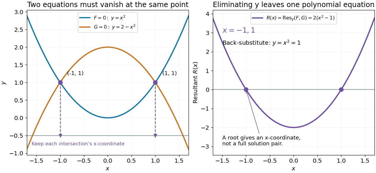
Polynomial elimination keeps the possible first coordinates of intersections
. Original parabola example. Left: both equations vanish at the two marked intersections; dashed lines retain their -coordinates on an auxiliary horizontal reference line at . Right: the resultant has zeros at those coordinates. Substitution recovers and verifies each full solution pair. Details.
In general, first solve the one-variable resultant equation, then recover and check the other coordinate in both original polynomial equations. A real coordinate candidate can correspond only to nonreal values of the eliminated variable. Also, vanishing leading coefficients require the separate check in degree drop in a specialized resultant. The general elimination-and-back-substitution method is described in the lecture's §3.1.[ref]
Lecture 6: Resultants and Discriminants. Algebraic Techniques and Semidefinite Optimization, MIT 6.972, Spring 2006; MIT 6.972, Lecture 6, p. 6-3, §3.1 Polynomial equations: eliminate one variable, solve and back-substitute
The actual-degree condition in the resultant theorem matters when coefficients depend on a parameter. TakeThe nominal degree-one Sylvester matrix is , whose determinant is . Its specialization at therefore vanishes. But the specialized polynomials are the nonzero constants and , which have no common root at all.
For , the roots of a polynomial are and ; neither has a finite limit as . Both leading coefficients vanish at the exceptional parameter. The fixed-size determinant has retained the original degree format even though the specialized polynomial degrees have dropped. Recompute using the actual specialized polynomials and check the original equations before accepting a zero of a parameter-dependent resultant as a solution.
Articles by others on the same topic
There are currently no matching articles.