The resultant turns a shared-root of a polynomial question into a calculation using only coefficients. For nonconstant univariate polynomials over a field , with their actual polynomial degrees , definewhere is the Sylvester matrix. ThenHere is an algebraic closure. The common root need not lie in : two real polynomials may share a nonreal complex root. The subscript identifies which variable is eliminated.[ref]
Lecture 6: Resultants and Discriminants. Algebraic Techniques and Semidefinite Optimization, MIT 6.972, Spring 2006; MIT 6.972, Lecture 6, 28 February 2006, pp. 6-1–6-2, Resultants: Sylvester matrix, root product and common-root criterion
The useful surprise is that a determinant detects a shared root of a polynomial without first finding either list of roots of a polynomial. If the coefficients depend on a parameter, the resultant itself is a polynomial in that parameter. Its zeros pick out possible exceptional parameter values. Elimination theory uses this to reduce a pair of polynomial equations in two variables to a single necessary equation in one variable; eliminating a variable with a resultant gives an exact example below.
A nonzero resultant also supplies a certificate that and are coprime polynomials. The Sylvester matrix then solves for polynomials satisfying , a Bézout's identity for polynomials. Evaluating such an identity at a hypothetical common root would give .
For polynomials of polynomial degrees , the Sylvester matrix has shifted coefficient rows of followed by shifted rows of , using descending-power order. It is a square matrix of size . Its transpose represents the linear map with , ; its determinant is the resultant.
For an original parameter example, choose and . ThenThe two lists of coefficients become three rows because is multiplied by both and . Thus the common-root parameter values are and . At , the resultant is , so the two polynomials have no common root.
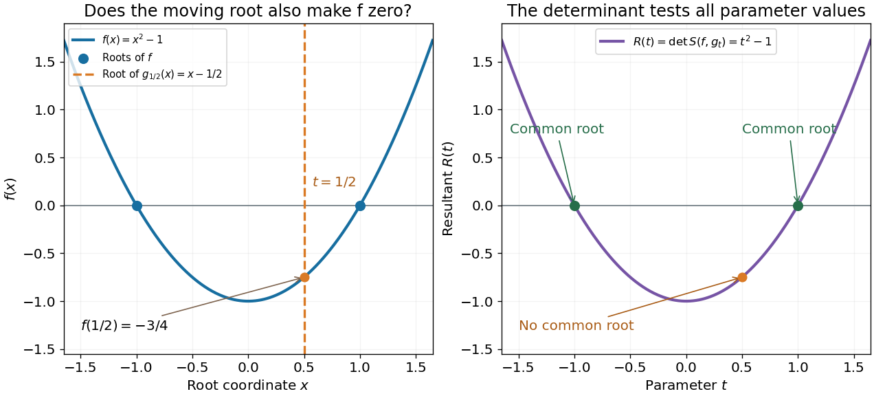
One can verify the certificate without any determinant expansion:For , division by gives a Bézout's identity for polynomials. At , the identity instead becomes a nontrivial cancellation between multiples of two polynomials sharing the polynomial factor .
The general proof needs only a short linear algebra outline. A common polynomial factor gives a nonzero cancelling pair within the degree bounds, making the Sylvester matrix singular. Conversely, if are coprime polynomials and , then divides ; the bound forces and then . Thus the linear map has zero kernel of a linear map exactly in the coprime case. Over an algebraic closure, a nonconstant common polynomial factor is equivalent to a common root.
In 1840, James Joseph Sylvester described forming the shifted coefficient rows and taking a signed sum of products selected by permutations. In modern notation, this is the Sylvester matrix and its determinant. The construction turns the nonlinear common-root of a polynomial question into linear algebra. His paper's word derivatives concerns elimination, rather than the formal derivative used below.[ref]
A method of determining by mere inspection the derivatives from two equations of any degree. The Collected Mathematical Papers of James Joseph Sylvester, Volume I; Paper 9, A method of determining by mere inspection the derivatives from two equations of any degree; Collected Mathematical Papers, volume I (1904), pp. 54–55, rules 1–4; original Philosophical Magazine XVI (1840), pp. 132–135
Write and in an algebraic closure, counting multiplicity of a root. The coefficient-row convention above givesThis makes the shared-root of a polynomial test transparent: a factor vanishes precisely when one equals one . Swapping the two polynomials reverses the sign of all differences, giving .[ref]
The value measures an algebraic product, not a normalized geometric distance. Replacing by for nonzero leaves its roots of a polynomial unchanged but multiplies the resultant by . Therefore a small numerical resultant alone does not quantify how close two sets of roots of a polynomial are. Exact zero testing and numerical sensitivity are different questions.
A multiple root of a polynomial is also a root of a polynomial of its formal derivative. In characteristic zero, for , the associated discriminant isFor example, gives and . The two roots of a polynomial merge precisely at .[ref]
Lecture 6: Resultants and Discriminants. Algebraic Techniques and Semidefinite Optimization, MIT 6.972, Spring 2006; MIT 6.972, Lecture 6, p. 6-2, Definition 2: discriminant as a polynomial–derivative resultant
Consider the original pair of polynomial equationsTreat them as polynomials in with coefficients in . Their Sylvester matrix and resultant areEvery common solution must therefore have or . Back-substitution into gives , and both pairs also satisfy . The complete real solution set isHere elimination and direct substitution agree: subtracting from gives , exactly the same condition.
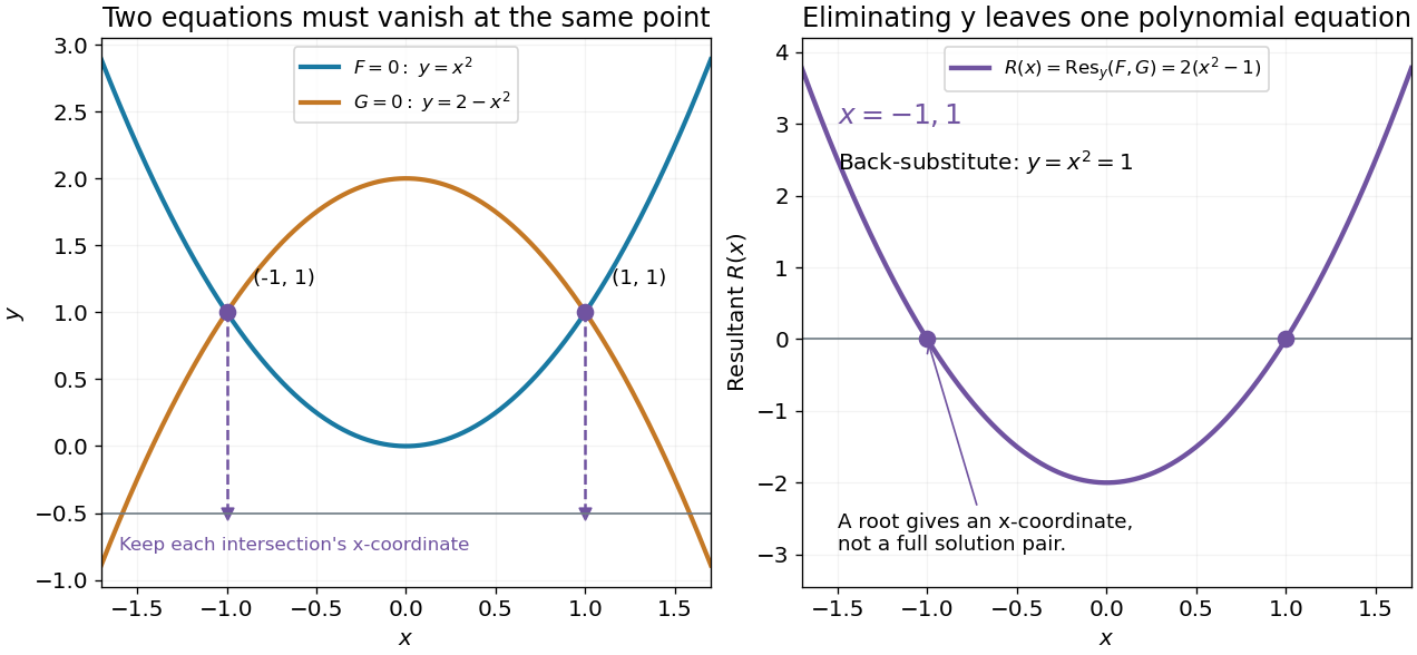
Polynomial elimination keeps the possible first coordinates of intersections
. Original parabola example. Left: both equations vanish at the two marked intersections; dashed lines retain their -coordinates on an auxiliary horizontal reference line at . Right: the resultant has zeros at those coordinates. Substitution recovers and verifies each full solution pair. Details.In general, first solve the one-variable resultant equation, then recover and check the other coordinate in both original polynomial equations. A real coordinate candidate can correspond only to nonreal values of the eliminated variable. Also, vanishing leading coefficients require the separate check in degree drop in a specialized resultant. The general elimination-and-back-substitution method is described in the lecture's §3.1.[ref]
Lecture 6: Resultants and Discriminants. Algebraic Techniques and Semidefinite Optimization, MIT 6.972, Spring 2006; MIT 6.972, Lecture 6, p. 6-3, §3.1 Polynomial equations: eliminate one variable, solve and back-substitute
The actual-degree condition in the resultant theorem matters when coefficients depend on a parameter. TakeThe nominal degree-one Sylvester matrix is , whose determinant is . Its specialization at therefore vanishes. But the specialized polynomials are the nonzero constants and , which have no common root at all.
For , the roots of a polynomial are and ; neither has a finite limit as . Both leading coefficients vanish at the exceptional parameter. The fixed-size determinant has retained the original degree format even though the specialized polynomial degrees have dropped. Recompute using the actual specialized polynomials and check the original equations before accepting a zero of a parameter-dependent resultant as a solution.
Articles by others on the same topic



The term "resultant" can refer to different concepts depending on the context in which it is used. Here are a few common interpretations: 1. **Vector Resultant**: In physics and mathematics, a resultant typically refers to a single vector that is equivalent to the combined effects of two or more vectors. For example, if two forces are acting at an angle to each other, the resultant force can be found using vector addition, which may involve graphical methods or mathematical calculations using trigonometry.