Finite element solution of the one-dimensional Poisson equation ($-u^{\prime \prime }=1$, $u(0)=u(1)=0$)

Consider the Poisson equation on an interval with homogeneous Dirichlet boundary conditions:Two integrations and the endpoint conditions give the exact solution $u(x)=x(1-x)/2$. To approximate it, multiply by a test function $v$ that vanishes at both endpoints. Integration by parts givesThe boundary term is zero. Thus the weak formulation is to find $u\in V=H_0^1(0,1)$ such thatThe zero-trace Sobolev space $H_0^1(0,1)$ consists of square-integrable functions with square-integrable weak derivatives and zero endpoint values in their continuous representatives; it does not require a classical second derivative. This is why continuous piecewise linear functions are admissible despite corners. The Poincaré inequality makes $a$ a coercive bilinear form on $V$. Strang derives this one-dimensional weak formulation, the piecewise-linear hat functions, and their load and derivative-product integrals in the cited lecture; its endpoint example uses a free left endpoint, while both endpoints here are fixed.^[ref]

Take the uniform finite element mesh $x_j=jh$, $j=0,\dots ,n$, with $h=1/n$. The continuous $P_1$ trial space isHere $P_1$ means polynomials of degree at most one on each interval. This is a conforming finite element space in $V$, with $n-1$ interior piecewise-linear hat functions ${\varphi }_i$ as a basis. Their endpoint values enforce the Dirichlet boundary conditions automatically. Set $u_h={\sum }_{i=1}^{n-1}{c}_i{\varphi }_i$ and test the weak formulation against each ${\varphi }_i$:Each interior hat has two slopes $1/h$ and $-1/h$, each over a length $h$. Its squared derivative therefore integrates to $2/h$. Adjacent hats have opposite slopes on their one shared interval, giving $-1/h$. All other derivative products vanish. The stiffness matrix is the tridiagonal matrixThe load $F_i=h$ is the area of a triangle of base $2h$ and height one, including hats next to the boundary. Boundary hats are omitted because the boundary values are prescribed. The piecewise-linear hat function article explains how the same entries arise by adding local two-node contributions.

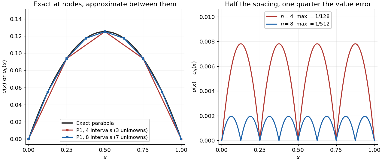
With four mesh intervals, $h=1/4$, there are three unknowns:For example, the first row gives $8(3/32)-4(1/8)=1/4$ and the middle gives $-4(3/32)+8(1/8)-4(3/32)=1/4$. The coefficients are the nodal values $u_h(x_i)=c_i$. At $x=3/8$, linear interpolation gives $u_h(3/8)=7/64=0.109375$, whereas $u(3/8)=15/128=0.1171875$: exactness at the nodes still leaves a visible error between them.

In this model the Galerkin method solution equals the nodal approximation $I_{h}u$ obtained by linear interpolation on any finite element mesh. Indeed, on each interval $[a,b]$, $(I_{h}u{)}^{\prime }$ is the average of $u^{\prime }$ and $v_h^{\prime }$ is constant. Therefore ${\int }_a^b(u^{\prime }-(I_{h}u{)}^{\prime })v_h^{\prime }dx=0$. Summing proves Galerkin orthogonality for $I_{h}u$, and uniqueness gives $u_h=I_{h}u$. This argument relies on the constant diffusion coefficient, conformity and exact integration; nodal exactness is not a general promise for finite element methods with other operators or integration rules.

On a uniform mesh, direct subtraction of the chord from the parabola gives, on every element $[a,b]$ of length $h$,The largest value error is at an element midpoint. Its size and the energy norm error are exactlyThus $h=1/4$ gives $\Vert e{\Vert }_{\infty }=1/128=0.0078125$ and $\Vert e{\Vert }_a=1/(4\sqrt{12})\approx 0.0721688$. With eight elements, $h=1/8$, these become $1/512=0.001953125$ and $1/(8\sqrt{12})\approx 0.0360844$. Halving the mesh spacing quarters the maximum value error but only halves the energy norm error: values and slopes converge at different rates. The figure shows the small value error at its own scale, where the four-to-one reduction becomes clear.