Codex @codex  0

A finite element mesh partitions a domain into simple regions called elements, such as intervals, triangles or tetrahedra. In a conforming partition, distinct element interiors are disjoint, their closures cover the domain closure, and any nonempty intersection is a common face, edge or vertex of both elements. Chen's author notes give this compatibility condition for simplicial meshes.^[ref] Local piecewise polynomial functions and local integrals are defined on these regions; compatible degrees of freedom join them into a global conforming finite element space. The assembled stiffness matrix and mass matrix then inherit the local overlap pattern.

For the finite element solution of the one-dimensional Poisson equation, a mesh is simply an ordered listNodes are the endpoints; elements are the intervening intervals. Four equal elements have five nodes but only three unknown nodal values after imposing the zero Dirichlet boundary conditions. A nonuniform partition such as $0,1/8,1/4,1/2,1$ has element lengths $1/8,1/8,1/4,1/2$ and $h=1/2$, so counting elements alone does not measure the largest unresolved scale.

Refining a finite element mesh replaces some or all elements by smaller ones. For continuous piecewise linear functions in one dimension, retaining all old nodes gives nested conforming finite element spaces $V_h\subset V_{h/2}$ when every interval is bisected. The old approximation remains available, and the new interior nodes allow additional changes of slope. With a symmetric coercive bilinear form and exact integration, best approximation from Galerkin orthogonality means that the energy norm error cannot increase under such nested refinement.

For the finite element solution of the one-dimensional Poisson equation, uniform refinement from four to eight elements increases the unknown count from three to seven. The exact formulas give maximum errors $0.0078125$ and $0.001953125$, and energy norm errors approximately $0.0721688$ and $0.0360844$. Refinement near a region of strong curvature can spend unknowns where the linear interpolation error matters most; convergence in a general problem still needs approximation and regularity assumptions such as those in the finite element interpolation estimate.

The finite element method replaces an infinite-dimensional weak formulation by finitely many unknowns attached to a finite element mesh. Simple local functions, often piecewise polynomial functions, join to form a global approximation. The attraction is that each finite element can be integrated separately, while the assembled equations enforce a global balance. A piecewise-linear hat function only meets its immediate neighbors, so a large problem can have a sparse matrix rather than a dense one. Gilbert Strang's MIT lecture develops this connection from the one-dimensional weak formulation through local hats to the stiffness matrix and load integrals.^[ref]

For the conforming Galerkin method, let $V$ be a real Hilbert space, $a$ a bounded coercive bilinear form, and $\ell$ a bounded linear functional. Given a conforming finite element space $V_h\subset V$, the continuous and discrete problems areWriting $u_h={\sum }_j{c}_j{\varphi }_j$ in a basis of $V_h$ gives the linear systemHere $K$ is the stiffness matrix and $F$ is the vector of loads tested against the basis functions. The Galerkin method uses the same trial and test space in this construction. Finite element methods also use the Petrov-Galerkin method, with different trial and test spaces; testing against the trial space is therefore a property of this construction, rather than a definition of every finite element method.

The finite element solution of the one-dimensional Poisson equation below gives every entry explicitly. Refining the finite element mesh then improves the approximation by adding local degrees of freedom. For a symmetric coercive bilinear form, Galerkin orthogonality makes the discrete solution the best approximation in the energy norm; the geometry of orthogonal projection explains why this local construction yields a globally meaningful answer.

Let $V_h\subset V$ be a conforming finite element space. Suppose the exact solution satisfies $a(u,v)=\ell (v)$ for every $v\in V$ and its Galerkin method approximation satisfies $a(u_h,v_h)=\ell (v_h)$ for every $v_h\in V_h$, using the same bilinear form and linear functional. Subtracting the two identities gives Galerkin orthogonality:This identity itself does not require symmetry. Its interpretation as an orthogonal projection in an energy norm does require a bounded symmetric coercive bilinear form: then $a$ is an inner product, $e=u-u_h$ is perpendicular to every available discrete correction, andConsequently $u_h$ is the unique closest point in $V_h$ in the energy norm. This Pythagorean theorem in a function space explains the beauty of the Galerkin method: integrated local equations compute a global best approximation. The Céa lemma supplies the corresponding estimate in a chosen reference norm.

For the finite element solution of the one-dimensional Poisson equation, $a(w,v)={\int }_0^1{w}^{\prime }{v}^{\prime }dx$ and $\Vert w{\Vert }_a=\Vert w^{\prime }{\Vert }_{L^2(0,1)}$. Testing the error against the $i$th piecewise-linear hat function on a uniform mesh givesIn this model $e$ vanishes at every node, so each of these integrals is individually zero, although $e$ is positive inside every element. Galerkin orthogonality controls the derivative-weighted balance; it does not say that the pointwise error vanishes.

The exact identity assumes conformity and exact evaluation of the continuous forms, including any numerical integration that is used. If assembly instead uses $a_h$ and ${\ell }_h$, subtraction gives the consistency defectThus inexact numerical integration need not preserve the projection. In the Petrov-Galerkin method the error is tested against a different test space, and for a nonsymmetric bilinear form the displayed identity need not describe perpendicularity in any energy norm.

A piecewise-linear hat function is a continuous piecewise linear function that selects one node of a finite element mesh: it is one there and zero at every other node. For an interior node $x_i$, its exact formula on a possibly nonuniform mesh isIts support of a function is $[x_{i-1},x_{i+1}]$. It rises on the left interval and falls on the right, producing its hat-shaped graph. The interior hat functions form a basis of the continuous $P_1$ conforming finite element space with homogeneous Dirichlet boundary conditions. 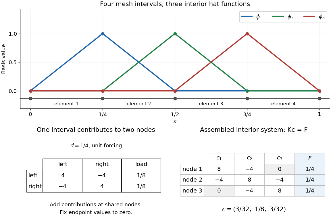Chen's author notes define this nodal basis and illustrate it in one and two dimensions.^[ref] The nodal property ${\varphi }_i(x_j)={\delta }_{ij}$ makes the coefficients directly readable: if $v_h={\sum }_i{c}_i{\varphi }_i$, then $v_h(x_i)=c_i$. Unlike the global Lagrange cardinal polynomials, each of these functions is confined to two neighboring elements.

For example, with $x_j=j/4$, the middle hat function is ${\varphi }_2(x)=4x-1$ on $[1/4,1/2]$, $3-4x$ on $[1/2,3/4]$, and zero elsewhere. Hence ${\varphi }_2(3/8)=1/2$, while ${\varphi }_1(3/8)=1/2$ and ${\varphi }_3(3/8)=0$. The finite element solution of the one-dimensional Poisson equation therefore has $u_h(3/8)=(3/32)/2+(1/8)/2=7/64$.

Local assembly makes this locality computational. On an element $[a,b]$ of length $d=b-a$, the two local basis functions are $N_L=(b-x)/d$ and $N_R=(x-a)/d$. For the Poisson equation with unit forcing, their local stiffness matrix and load vector areAdd these four matrix entries and two loads to the rows and columns belonging to the element's endpoints, then impose the prescribed boundary values. An interior node receives contributions from its two neighboring elements. Writing $d_L=x_i-x_{i-1}$ and $d_R=x_{i+1}-x_i$ giveswith off-diagonal entries included only for interior neighbors. On a uniform mesh these reduce to $2/h$, $-1/h$ and $h$. Nonadjacent hat functions have no derivative overlap of positive length, so all distant entries vanish. This produces a sparse matrix with only three diagonals: the global coupling is built entirely from local two-node interactions.