Flow-profile mismatch in Doppler stroke-volume estimation

Flow-profile mismatch in Doppler stroke-volume estimation occurs when the velocity used in a stroke volume calculation does not represent the spatial average over the measured opening. The exact instantaneous volumetric flow rate isfor fixed area $A$. Consequently $\mathrm{SV}=A\int \bar{v}(t)dt$. Replacing $\bar{v}$ by a centerline velocity or fastest spectral envelope requires an additional profile assumption. The ASE report distinguishes the modal part of a pulsed Doppler spectrum from the outer continuous-wave envelope representing the fastest detected cells.^[ref]

An original family of axisymmetric profiles makes the missing factor explicit. Within a circular opening of radius $R$, supposeHere $u(t)$ is the centerline velocity. Integrating concentric annuli givesThe Doppler profile correction factor is therefore $\alpha =n/(n+2)$ for this stipulated family. A parabolic profile $n=2$ has $\alpha =1/2$; a blunter profile $n=8$ has $\alpha =0.8$. Both have the same centerline velocity and vanish at the wall. These shapes are examples, not fitted cardiac profiles.

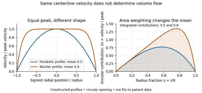
For $R=1\mathrm{cm}$ and a centerline velocity-time integral of $20\mathrm{cm}$, uncorrected multiplication by $A=\pi \mathrm{c}{\mathrm{m}}^2$ gives $62.8\mathrm{mL}$. The two model profiles instead transport approximately $31.4$ and $50.3\mathrm{mL}$. Identical peak data can therefore support different transported volumes when the profile differs.

Real Doppler measurements also involve beam direction, sample-volume extent and signal processing. Their spectral envelope need not coincide with the literal centerline trace used in this example. The illustration isolates the averaging issue; it is not a universal factor-of-two correction for clinical measurements. The sampling site and anatomical area must be matched as well.^[ref]

A Doppler profile correction factor converts a specified sampled velocity into the area-mean normal velocity needed to calculate volumetric flow rate. For a fixed opening of cross-sectional area $A$ and nonzero sampled trace $u_s(t)$, defineThe definition depends on both the spatial flow profile and what the instrument's sampled trace represents. A centerline trace, spectral mode and fastest detected envelope need not have the same correction. The primary ASE report distinguishes these spectral quantities and requires matched locations for velocity and area measurements.^[ref]

Even if each instantaneous correction is known, the appropriate correction for a whole velocity-time integral is generally not its ordinary time average. Provided the denominator is nonzero,This velocity-weighted Doppler profile correction gives greater influence to intervals carrying more of the sampled velocity-time integral.

In an original two-interval calculation, each interval lasts one second. Let sampled velocities be 10 and 30 cm/s and instantaneous corrections 0.5 and 1.0. The sampled velocity-time integral is 40 cm, while its corrected counterpart is $0.5\times 10+1\times 30=35$ cm. Thus ${\alpha }_{\mathrm{eff}}=0.875$, whereas the ordinary average correction is 0.75. For $A=1\mathrm{c}{\mathrm{m}}^2$, the latter would predict 30 mL instead of the model's 35 mL.

When the sampled velocity is nonnegative, this is a weighted mean and lies between the instantaneous corrections. Reversing fluid flow can create cancellation in the denominator, so that conclusion need not hold. A factor measured in a steady tube also cannot be assigned to a changing cardiac profile without evidence. The calculation explains an averaging requirement; it supplies no universal clinical correction.

A velocity-weighted Doppler profile correction converts an integrated sampled velocity into an integrated area-mean velocity by weighting each instantaneous correction according to the sampled velocity at that time. For a fixed opening of cross-sectional area $A$, suppose its area-mean normal velocity is $\bar{v}(t)=\alpha (t)u(t)$. Thenprovided the denominator is nonzero. Applying the time average of $\alpha$ to a velocity-time integral generally answers a different question.

The error has an exact covariance form. Define $⟨g⟩=T^{-1}{\int }_0^{T}g(t)dt$ and time covariance ${\mathrm{Cov}}_t(\alpha ,u)=⟨\alpha u⟩-⟨\alpha ⟩⟨u⟩$. ThenConsequently an unweighted correction is exact if that covariance vanishes, even when the correction varies in time. Its failure is about how profile changes align with transport, not merely whether either trace varies.

In an original two-second example, equal one-second intervals have sampled velocities 10 and 40 cm/s and corrections 1.0 and 0.5. The unweighted mean correction is 0.75, but ${\alpha }_{\mathrm{eff}}=(10+20)/50=0.60$. With $A=2\mathrm{c}{\mathrm{m}}^2$, actual modeled transport is 60 mL; unweighted correction predicts 75 mL, a 25% overestimate. Here time covariance is $-3.75$ cm/s and mean sampled velocity is 25 cm/s, recovering $0.75-3.75/25=0.60$.

If $u$ is nonnegative, normalized velocity weights are nonnegative and ${\alpha }_{\mathrm{eff}}$ lies between the instantaneous corrections. For reversing fluid flow, the denominator can instead approach zero through cancellation. Forward and reverse transported volumes can then be more informative than a single unstable ratio. If opening area changes, the integral must also retain $A(t)$; this fixed-area correction does not remove that additional dependence.

The primary Doppler report requires appropriate matching of sampled velocity and anatomical area and distinguishes modal spectral velocities from the fastest envelope.^[ref] The covariance calculation is an original integration identity, not a universal clinical profile correction.