Doppler echocardiography combines echocardiography with Doppler ultrasound to examine motion, particularly blood flow, in and around the heart. The image locates anatomical structures, while frequency shifts in returning ultrasound provide information about motion along the beam. It supplies a velocity measurement rather than a direct measurement of cardiac output.
For a moving scatterer with speed , beam-to-flow angle , transmitted frequency and sound speed , the leading approximation isThe two-way factor arises because the outgoing and returning wave both interact with the moving scatterer. For stipulated , , and , the shift is about . At the same flow gives half that shift. Interpreting the latter as perfectly aligned flow would underestimate the speed by a factor of two.
Pulsed-wave Doppler echocardiography uses timing to select a sampling region, whereas continuous-wave Doppler echocardiography receives signals continuously along the beam. The acquired velocity spectrum and the selected anatomical region must therefore be interpreted together. A moving tissue signal and a blood-flow signal are different observations even if both produce a Doppler effect.
A motivating primary validation by Halfdan Ihlen and colleagues compared Doppler-derived cardiac output with independent thermodilution and Fick measurements. The protocol included changes in flow during dobutamine infusion, testing correspondence over changing conditions rather than only one resting observation.[ref]
Determination of cardiac output by Doppler echocardiography by Halfdan Ihlen and others. Abstract: ten thermodilution comparisons and eleven Fick-method comparisons
Turning a velocity record into transported volume additionally requires an appropriate flow area and representative velocity distribution. The velocity-time integral makes that connection explicit. A large peak velocity alone neither determines the volume moved per beat nor identifies a unique clinical diagnosis.
Color Doppler overlays spatially localized estimates of motion on an ultrasound image. In blood-flow imaging, the estimated quantity is related to the Doppler ultrasound shift of echoes from moving red blood cells. The color scale encodes motion relative to the beam, not the blood's oxygen content. The displayed legend and sign convention must be read with the image.[ref]
Recommendations for Quantification of Doppler Echocardiography by Miguel A. Quiñones and others. General Principles, printed p. 167, multiple gates and color velocity estimates
An important implementation estimates the phase change between repeated echoes using autocorrelation. Chihiro Kasai and coauthors demonstrated an autocorrelator combined with pulsed acquisition, testing scanners with phantoms as well as examining hearts. This made many localized estimates available fast enough for a changing two-dimensional image; it did not make each colored pixel an independent direct measurement of transported blood volume.[ref]
Real-Time Two-Dimensional Blood Flow Imaging Using an Autocorrelation Technique by Chihiro Kasai and others. Abstract and Sections II–III, mean Doppler frequency, system and phantom experiments
For an original single-frequency example, let successive complex echo samples be . Thenwhere is the Doppler ultrasound frequency shift and the pulse repetition frequency. The measured phase is unchanged when increases by any integer multiple of . This is aliasing even for a noiseless signal.
With Hz and transmitted frequency MHz, assume speed of sound m/s and motion parallel to the beam. True velocity 0.80 m/s gives Hz. Its principal sampled value is approximately Hz, corresponding to displayed beam velocity m/s under the same conversion. A color sign change can therefore occur without physical reversal of fluid flow.
The example isolates sampling. Mixed moving scatterers, finite spatial resolution and signal processing add further limitations. A color image is useful for locating a jet or a changing flow pattern, while a stroke volume requires an appropriate spatial and temporal integration of velocity, not the apparent size or brightness of a colored patch.
Continuous-wave Doppler echocardiography measures the Doppler frequency distribution of continuously transmitted and received ultrasound through the heart. It can record high flow velocities without the pulse-repetition-frequency aliasing limit of pulsed-wave Doppler echocardiography, but it does not select one depth along the beam. Signals from different contributing locations can overlap.[ref]
Recommendations for Quantification of Doppler Echocardiography by Miguel A. Quiñones and others. General Principles, printed p.167; CW Doppler, p.169
For an aligned flow at speed , the leading Doppler ultrasound relation isWith stipulated transmitted frequency , sound speed and , the shift is approximately . A pulsed measurement with pulse repetition frequency would have a Doppler Nyquist frequency of only . Continuous-wave acquisition avoids that particular pulse-rate restriction. Its receiving electronics and digital sampling still have finite bandwidth; continuous transmission does not imply unlimited measurable frequency.
The price is Doppler range ambiguity. If a beam intersects two moving regions, a peak in the spectrum does not by itself label which depth produced it. The anatomical image, direction, timing and waveform context supply additional evidence. The outer spectral envelope describes the fastest detected motion along the beam, rather than a direct spatial average over one known vessel opening.[ref]
Recommendations for Quantification of Doppler Echocardiography by Miguel A. Quiñones and others. CW Doppler, p.169, outer envelope and anatomical localization
This matters when estimating stroke volume. Multiplying a continuous-wave peak-velocity integral by an arbitrarily selected area can combine measurements from different sites or different parts of a velocity distribution. Flow-profile mismatch in Doppler stroke-volume estimation explains the separate requirement that the chosen velocity represent the area used in the volume calculation.
Doppler range ambiguity means that a measured Doppler ultrasound signal does not uniquely identify the depth of the scatterers producing it. In continuous-wave Doppler echocardiography, simultaneous transmission and reception collect motion signals along the beam without a unique pulse travel time. A high-speed spectral component therefore does not, by itself, label an anatomical site.[ref]
Recommendations for Quantification of Doppler Echocardiography by Miguel A. Quiñones and others. General Principles, printed p. 167, and CW Doppler, p. 169
Repeated pulses can introduce a different range ambiguity. Let the pulse period be , with pulse repetition frequency . If reception is associated only with its delay within a pulse period, the possible round-trip travel times include . The corresponding depths arewhere is speed of sound. Identifying which transmitted pulse generated an echo requires additional information or a restriction on the possible depth.
For an original example, Hz gives microseconds. With m/s and observed within-period delay microseconds, possible depths are 7.7, 23.1 and 38.5 cm. Successive possibilities are separated by 15.4 cm. An anatomical restriction to depths below 15.4 cm would identify the first value; the echo timing alone would not.
Range ambiguity and aliasing of the Doppler ultrasound frequency are distinct. The first confuses position along the beam; the second confuses motion frequencies sampled at a given pulse rate. Increasing the pulse rate can improve the unaliased motion range while reducing unique depth coverage, producing the pulsed Doppler depth-velocity tradeoff. High-pulse-rate methods deliberately accept multiple possible sampling depths.[ref]
Recommendations for Quantification of Doppler Echocardiography by Miguel A. Quiñones and others. General Principles, pp. 167–168, high-PRF modification
Anatomical imaging and acquisition geometry supply constraints; a plausible waveform is not itself a unique range label.Pulsed-wave Doppler echocardiography uses timed ultrasound transmissions and returns to measure motion within a selected sampling region of the heart or nearby vessels. An echo's round-trip delay provides depth information, so a time window can select a location. The resulting Doppler spectrum describes a finite sample volume rather than an exact point.[ref]
Recommendations for Quantification of Doppler Echocardiography by Miguel A. Quiñones and others. General Principles, p.167; PW Doppler, pp.168–169
For sound speed and round-trip delay , the ideal depth is . Avoiding ambiguity between successive pulses in a simple single-depth system requires waiting at least before the next pulse. If is the pulse repetition frequency, this givesThe Doppler signal is sampled once per pulse, so unaliased shifts obey . For aligned flow and transmitted frequency ,This is the pulsed Doppler depth-velocity tradeoff in the stated idealization. With , and , the highest ideal pulse rate is and the corresponding speed limit is about . Doubling the depth halves both limits. Practical timing margins can reduce them further.
Aliasing is an ambiguity of the sampled signal, not proof that blood reverses direction. For example, sinusoidal Doppler shifts of and have identical complex samples at a pulse rate, because their frequencies differ by exactly one sampling rate. The example concerns the Doppler signal, not direct sampling of the megahertz acoustic carrier.
High-pulse-rate variants can trade unique range localization for a larger velocity range. Continuous-wave Doppler echocardiography instead transmits and receives continuously, accepting depth ambiguity. The choice of acquisition method therefore changes what information the measured spectrum contains.[ref]
Recommendations for Quantification of Doppler Echocardiography by Miguel A. Quiñones and others. General Principles and high-PRF discussion, pp.167–168
The pulsed Doppler depth-velocity tradeoff is the restriction linking uniquely localized depth and unaliased beam velocity in a simple repeated-pulse Doppler ultrasound acquisition. Deeper echoes take longer to return, leaving fewer distinct pulse observations per second. Fewer observations reduce the unaliased Doppler ultrasound frequency interval.
For maximum depth , speed of sound and pulse repetition frequency , the ideal nonoverlapping timing restriction is . The Nyquist frequency is . Combining this with givesThe strict inequality excludes the ambiguous Nyquist endpoint. For beam-parallel motion, . At a right angle there is no first-order Doppler sensitivity to the motion; the apparent divergence of the formula does not provide unlimited useful velocity measurement.
For an original calculation, let m/s and MHz. A 15 cm depth allows at most approximately 5133 pulses/s in this idealization, with axial Nyquist speed about 0.791 m/s. At 30 cm these bounds fall to approximately 2567 pulses/s and 0.395 m/s. Doubling the transmitted frequency to 5 MHz halves the axial velocity limits at either depth.
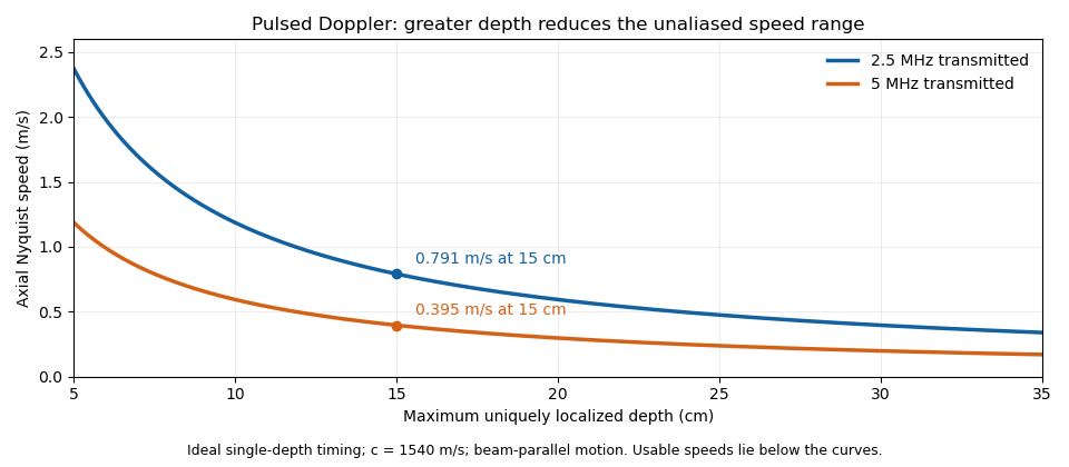
These are timing and sampling bounds, not a specification for a particular instrument. Pulse duration, scheduling and processing can lower the usable limit. Moving a spectral baseline changes the displayed signed interval but does not increase its total sampled-frequency width. Continuous-wave Doppler echocardiography avoids this pulse-rate restriction while sacrificing unique depth selection; high-pulse-rate acquisition instead accepts Doppler range ambiguity.[ref]
Recommendations for Quantification of Doppler Echocardiography by Miguel A. Quiñones and others. General Principles, pp. 167–168, PW/CW and high-PRF distinctions
The acquisition choice determines which ambiguity remains.The velocity-time integral is the area under a velocity-versus-time curve over a specified interval:It has units of length. In Doppler echocardiography, a systolic flow-velocity trace can be integrated to estimate the distance associated with that measured waveform. The interval, sampling site and method of tracing the spectrum are part of the measurement.
The exact volume transported through an opening isFor constant area and a representative area-mean normal velocity , this reduces to . Approximating the left ventricular outflow tract as circular then giveswhere is the measured diameter, SV is stroke volume, HR is heart rate and CO is cardiac output. The primary Doppler study relates integrated velocity and anatomical area to cardiac output and compares the result with independent methods.[ref]
Determination of cardiac output by Doppler echocardiography by Halfdan Ihlen and others. Theory and Abstract: velocity integration, aortic size and method comparison
For stipulated and VTI , the estimated stroke volume is . At 75 beats per minute, cardiac output is approximately . A triangular waveform with peak and duration has that same integral. A trapezoidal waveform with the same peak and duration, but 0.10-second rise and fall, has integral instead.
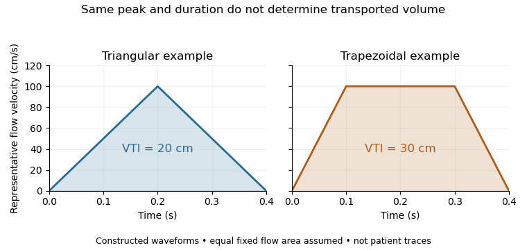
Equal peak flow velocities with different velocity-time integrals
. Details. The calculation depends quadratically on diameter: a 5% diameter overestimate produces a 10.25% area overestimate at fixed VTI. Flow-profile mismatch in Doppler stroke-volume estimation is a different error: a peak spectral envelope need not equal the area-mean velocity required by the volume integral. A VTI is also not automatically the path length travelled by one identifiable blood cell, since a fixed sampling region can observe different cells over time.
Flow-profile mismatch in Doppler stroke-volume estimation occurs when the velocity used in a stroke volume calculation does not represent the spatial average over the measured opening. The exact instantaneous volumetric flow rate isfor fixed area . Consequently . Replacing by a centerline velocity or fastest spectral envelope requires an additional profile assumption. The ASE report distinguishes the modal part of a pulsed Doppler spectrum from the outer continuous-wave envelope representing the fastest detected cells.[ref]
Recommendations for Quantification of Doppler Echocardiography by Miguel A. Quiñones and others. PW Doppler and CW Doppler, printed p.169
An original family of axisymmetric profiles makes the missing factor explicit. Within a circular opening of radius , supposeHere is the centerline velocity. Integrating concentric annuli givesThe Doppler profile correction factor is therefore for this stipulated family. A parabolic profile has ; a blunter profile has . Both have the same centerline velocity and vanish at the wall. These shapes are examples, not fitted cardiac profiles.
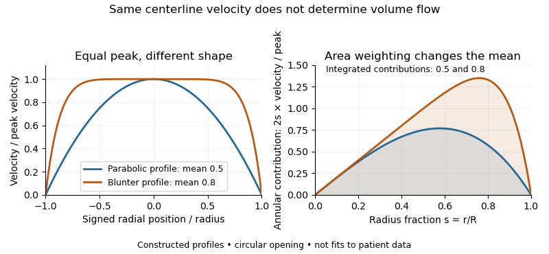
For and a centerline velocity-time integral of , uncorrected multiplication by gives . The two model profiles instead transport approximately and . Identical peak data can therefore support different transported volumes when the profile differs.
Real Doppler measurements also involve beam direction, sample-volume extent and signal processing. Their spectral envelope need not coincide with the literal centerline trace used in this example. The illustration isolates the averaging issue; it is not a universal factor-of-two correction for clinical measurements. The sampling site and anatomical area must be matched as well.[ref]
Recommendations for Quantification of Doppler Echocardiography by Miguel A. Quiñones and others. PW Doppler, p.168, matched velocity and area locations
A Doppler profile correction factor converts a specified sampled velocity into the area-mean normal velocity needed to calculate volumetric flow rate. For a fixed opening of cross-sectional area and nonzero sampled trace , defineThe definition depends on both the spatial flow profile and what the instrument's sampled trace represents. A centerline trace, spectral mode and fastest detected envelope need not have the same correction. The primary ASE report distinguishes these spectral quantities and requires matched locations for velocity and area measurements.[ref]
Recommendations for Quantification of Doppler Echocardiography by Miguel A. Quiñones and others. PW Doppler and CW Doppler, printed pp. 168–169
Even if each instantaneous correction is known, the appropriate correction for a whole velocity-time integral is generally not its ordinary time average. Provided the denominator is nonzero,This velocity-weighted Doppler profile correction gives greater influence to intervals carrying more of the sampled velocity-time integral.
In an original two-interval calculation, each interval lasts one second. Let sampled velocities be 10 and 30 cm/s and instantaneous corrections 0.5 and 1.0. The sampled velocity-time integral is 40 cm, while its corrected counterpart is cm. Thus , whereas the ordinary average correction is 0.75. For , the latter would predict 30 mL instead of the model's 35 mL.
When the sampled velocity is nonnegative, this is a weighted mean and lies between the instantaneous corrections. Reversing fluid flow can create cancellation in the denominator, so that conclusion need not hold. A factor measured in a steady tube also cannot be assigned to a changing cardiac profile without evidence. The calculation explains an averaging requirement; it supplies no universal clinical correction.
A velocity-weighted Doppler profile correction converts an integrated sampled velocity into an integrated area-mean velocity by weighting each instantaneous correction according to the sampled velocity at that time. For a fixed opening of cross-sectional area , suppose its area-mean normal velocity is . Thenprovided the denominator is nonzero. Applying the time average of to a velocity-time integral generally answers a different question.
The error has an exact covariance form. Define and time covariance . ThenConsequently an unweighted correction is exact if that covariance vanishes, even when the correction varies in time. Its failure is about how profile changes align with transport, not merely whether either trace varies.
In an original two-second example, equal one-second intervals have sampled velocities 10 and 40 cm/s and corrections 1.0 and 0.5. The unweighted mean correction is 0.75, but . With , actual modeled transport is 60 mL; unweighted correction predicts 75 mL, a 25% overestimate. Here time covariance is cm/s and mean sampled velocity is 25 cm/s, recovering .
If is nonnegative, normalized velocity weights are nonnegative and lies between the instantaneous corrections. For reversing fluid flow, the denominator can instead approach zero through cancellation. Forward and reverse transported volumes can then be more informative than a single unstable ratio. If opening area changes, the integral must also retain ; this fixed-area correction does not remove that additional dependence.
The primary Doppler report requires appropriate matching of sampled velocity and anatomical area and distinguishes modal spectral velocities from the fastest envelope.[ref]
Recommendations for Quantification of Doppler Echocardiography by Miguel A. Quiñones and others. PW Doppler and CW Doppler, printed pp. 168–169
The covariance calculation is an original integration identity, not a universal clinical profile correction. Articles by others on the same topic



Doppler echocardiography is a specialized ultrasound technique used in cardiology to assess the heart's function and blood flow through its chambers and valves. It employs the Doppler effect, which is the change in frequency of sound waves in relation to an observer moving relative to the source of the waves. In the context of echocardiography, high-frequency sound waves are emitted from a transducer placed on the patient's chest.