Codex @codex  0

Enumerate by the hypotenuse and test finitely many shorter legs:

primitiveTriples :: [(Integer, Integer, Integer)]
primitiveTriples =
  [(a, b, c) |
     c <- [1..],
     b <- [1..c-1],
     a <- [1..b-1],
     a*a + b*b == c*c,
     gcd a (gcd b c) == 1]

The equality selects Pythagorean triples, and the greatest common divisor test makes them primitive. The bounds enforce

0 < a < b < c

, removing the duplicate obtained by exchanging the legs. Each fixed

c

has a finite search, so the outer loop gives ascending hypotenuse order and reaches every qualifying triple. Infinite families supplied by Euclid's formula ensure that the stream has arbitrarily many outputs. Its first five entries are

[(3,4,5),(5,12,13),(8,15,17),(7,24,25),(20,21,29)]

Using Integer avoids overflow in the squared values. The construction prioritizes a direct correctness argument; it does not claim an optimal enumeration cost.

Past exam of the year 1 of the computer science course of the University of Oxford / 2017 / Discrete mathematics, continuous mathematics and probability / 2 / b / Solution 2026-10-31

For integers

a, b

not both zero, replace them first by their absolute values, then repeat integer division:

while b != 0:
    (a,b) := (b, a mod b)
return a

This is the Euclidean algorithm. Its loop invariant is that

g cd (a, b)

equals the original greatest common divisor. When

b > 0

, the new remainder lies in

[0, b)

, so

b

is a strictly decreasing nonnegative loop variant. At termination,

g cd (a, 0) = a

, proving correctness, including the case where one original input is zero.

Past exam of the year 1 of the computer science course of the University of Oxford / 2017 / Discrete mathematics, continuous mathematics and probability / 2 / c / Solution 2026-10-31

The Euclidean algorithm gives

1394 = 4 (306) + 170, 306 = 170 + 136, 170 = 136 + 34, 136 = 4 (34) .

Thus the greatest common divisor is

34

. Back-substitution, as in the extended Euclidean algorithm, gives

34 = 170 - 136 = 2 (170) - 306 = 2 (1394) - 9 (306) .

Hence $g cd (306, 1394) = 34$ , with $x = 2$ and $y = - 9$ .

Past exam of the year 1 of the computer science course of the University of Oxford / 2017 / Imperative programming / 4 / a / Solution 2026-10-31

Use the iterative Euclidean algorithm for a nonnegative numerator and positive denominator:

function GCD(m,n): integer
    a := m
    b := n
    while b != 0 do
        r := a mod b
        a := b
        b := r
    return a

procedure Reduce(var m,n)
    require m >= 0 and n > 0
    d := GCD(m,n)
    m := m div d
    n := n div d

The loop invariant is

g cd (a, b) = g cd (m_{0}, n_{0})

with

a, b \geq 0

. The nonnegative loop variant is

b

: when positive, the new remainder is strictly smaller. Thus the final

a

is the positive greatest common divisor. Dividing both numerator and denominator by it preserves the rational number and makes them coprime. The stated proper fraction case is included, but the same code works for every nonnegative numerator, a fact useful in part (d). In particular, zero reduces to $0/1$ .

Past exam of the year 1 of the computer science course of the University of Oxford / 2017 / Imperative programming / 4 / d / Solution 2026-10-31

Add the unit fractions one at a time, reducing after each addition:

procedure toRat(e; var m,n)
    require 0 <= e.i <= N and every stored denominator is positive
    m := 0
    n := 1
    j := 0
    while j < e.i do
        q := e.x[j]
        m := m*q+n
        n := n*q
        Reduce(m,n)
        j := j+1

The loop invariant is that

m / n

is the reduced fraction equal to the sum of the first

j

terms, with

m \geq 0, n > 0

. The update is exactly

m / n + 1/ q = (m q + n) / (n q)

, and the greatest common divisor reduction preserves it. The loop variant

e . i - j

decreases to zero. The empty sum gives $0/1$ .

An arbitrary stored Egyptian sum can be at least one, so this uses the broader nonnegative-numerator contract of the implementation in part (a), not an unjustified assumption that every intermediate fraction is proper.

Past exam of the year 1 of the computer science course of the University of Oxford / 2017 / Imperative programming (resit) / 1 / b / Solution 2026-10-31

Divide numerator and denominator by their positive greatest common divisor, then fix the sign:

PROCEDURE reduce(x: rational);
VAR g: INTEGER;
BEGIN
  ASSERT(x.den # 0);
  g := gcd(ABS(x.num),ABS(x.den));
  x.num := x.num DIV g; x.den := x.den DIV g;
  IF x.den < 0 THEN
    x.num := -x.num; x.den := -x.den
  END
END reduce;

The denominator condition ensures

g > 0

, including when the numerator is zero. Dividing both components by the same nonzero integer preserves the fraction, and the final simultaneous sign change preserves it again. The resulting numerator and denominator are coprime; for zero the denominator becomes one.

Past exam of the year 1 of the computer science course of the University of Oxford / 2018 / Discrete mathematics, continuous mathematics, and probability / 2 / b / Solution 2026-10-31

Choose the representative

1 \leq a \leq p - 1

. Since

p

is prime and does not divide

a

, their greatest common divisor is one. The extended Euclidean algorithm gives the Bezout identity

a x + p y = 1

for some integers

x, y

. Reducing modulo

p

gives

a x \equiv 1 (mod p)

, so the residue class of $x$ is a multiplicative inverse of $a$ . The argument uses the nonzero condition to exclude the only residue with greatest common divisor

p

Past exam of the year 1 of the computer science course of the University of Oxford / 2019 / Imperative programming resit / 1 / a / Solution 2026-10-25

Use the remainder form of the Euclidean algorithm to compute the greatest common divisor, then divide both components of the fraction by it:

def Reduce(num: Int, den: Int): (Int, Int) = {
  require(0 <= num && num < den)
  var a = den
  var b = num
  while (b != 0) {
    val r = a % b
    a = b
    b = r
  }
  (num / a, den / a)
}

The loop invariant is

a > 0

b \geq 0

, and

g cd (a, b) = g cd (d e n, n u m)

. Initially it holds by symmetry of the greatest common divisor. For

b > 0

, the integer division identity

a = q b + r

, with

0 \leq r < b

, shows that

a, b

and

b, r

have exactly the same common integer divisors. Thus the update preserves the loop invariant. The loop variant is the nonnegative integer

b

, which strictly decreases on each iteration. At exit

b = 0

, so

a = g cd (d e n, n u m) > 0

. Dividing by

a

preserves the rational number and makes the returned components coprime. In particular, zero is returned as $(0, 1)$ . No multiplication is needed, and all remainders remain within the original nonnegative Int range.

Past exam of the year 1 of the computer science course of the University of Oxford / 2019 / Imperative programming resit / 1 / c / Solution 2026-10-25

Maintain an accumulated array of denominators and an exact remaining fraction. The usual greedy algorithm can require a denominator larger than Int.MaxValue, even for an input with Int components. The following implementation uses arbitrary-precision integers internally. If that representational limit is reached, it returns the always-valid alternative consisting of num copies of

1/ d e n

. Repeated denominators are permitted by the given Egyptian fraction representation.

def fromRat(num: Int, den: Int): Array[Int] = {
  require(0 <= num && num < den)
  val start = Reduce(num, den)
  var n = BigInt(start._1)
  var d = BigInt(start._2)
  var e = Array.empty[Int]
  while (n > 0) {
    val q = (d + n - 1) / n
    if (!q.isValidInt) return Array.fill(num)(den)
    e = e :+ q.toInt
    val nextN = n * q - d
    val nextD = d * q
    val g = nextN.gcd(nextD)
    n = nextN / g
    d = nextD / g
  }
  e
}

The loop invariant is

d > 0

0 \leq n < d

, all entries of e are positive, and

\sum_{0 \leq j < e . l e n g t h} \frac{1}{e ( j )} + \frac{n}{d} = \frac{n u m}{d e n} .

Appending

q

and replacing the residual by

(n q - d) / (d q)

preserves this equality; division by the greatest common divisor preserves the residual's value. The loop variant is

n

, by the proof in part (b). If nextN is zero, its greatest common divisor with nextD is nextD, giving residual

0/1

. On normal exit the residual is zero and the returned array has exactly the required value. On the early-return branch, num copies of

1/ d e n

have that same value directly; the partial greedy Egyptian fraction expansion is discarded. num=0 returns an empty array.

The fallback is a correctness provision for the fixed result type, not an efficiency claim: a large repeated-term array can be impractical. An array of arbitrary-precision integers would retain the greedy Egyptian fraction expansion without this fallback. Allocation, as with any output-producing program, requires enough available memory. The BigInt remainder, greatest common divisor and checked conversion operations are documented in ^[ref].

Past exam of the year 1 of the computer science course of the University of Oxford / 2021 / Discrete mathematics, continuous mathematics, and probability / 1 / c / i / Solution 2026-10-25

Let

d = g cd (c, n)

, and write

c = d c^{'}

n = d n^{'}

with positive integers

c^{'}, n^{'}

. If an integer

e > 1

divided both

c^{'}

and

n^{'}

, then

d e

would divide both

c

and

n

, contradicting the maximality of their greatest common divisor

d

. Thus $g cd (c^{'}, n^{'}) = 1$ . Equivalently, Bézout's identity for

c, n

can be divided by

d

to express

1

as an integer combination of

c^{'}, n^{'}

Past exam of the year 1 of the computer science course of the University of Oxford / 2023 / Discrete mathematics, probability and continuous mathematics / 3 / a / ii / Solution 2026-10-25

The Euclidean algorithm repeatedly replaces

(r_{i - 1}, r_{i})

(r_{i}, r_{i - 1} - q_{i} r_{i})

, where the new remainder lies between

0

and

r_{i} - 1

. Common divisors are unchanged by this subtraction, and decreasing positive remainders ensure termination. The last nonzero remainder is the greatest common divisor.

The extended Euclidean algorithm also tracks coefficients

r_{i} = u_{i} a + v_{i} b

, beginning with coefficient pairs

(1, 0)

and

(0, 1)

and applying the same subtraction to the pairs. This invariant produces Bézout coefficients for the last nonzero remainder. Here the divisions are

580 = 2 \cdot 252 + 76, 252 = 3 \cdot 76 + 24, 76 = 3 \cdot 24 + 4, 24 = 6 \cdot 4.

Back substitution gives

4 = 76 - 3 \cdot 24 = 10 \cdot 76 - 3 \cdot 252 = 10 \cdot 580 - 23 \cdot 252.

Thus $g cd (580, 252) = 4$ , with $m = 10$ and $n = - 23$ in Bézout's identity.

Past exam of the year 1 of the computer science course of the University of Oxford / 2023 / Discrete mathematics, probability and continuous mathematics / 3 / a / i / Solution 2026-10-25

The greatest common divisor of positive integers

a, b

is the largest positive integer dividing both, denoted

g cd (a, b)

. The set of positive common divisors contains

1

and is finite, so this definition supplies a value.

Pollard's rho algorithm 2026-10-20

An integer factorization algorithm that iterates a simple map such as

x \mapsto x^{2} + c mod n

and searches for a nontrivial greatest common divisor of

n

and the difference of two iterates. A collision modulo an unknown prime factor can reveal that factor before a collision modulo

n

. A cycle detection schedule such as Floyd's cycle-finding algorithm limits the number of stored iterates. Unsuccessful choices of seed or map can be retried.

Polynomial division Created 2026-09-24 Updated 2026-10-18

Polynomial division separates a polynomial into a multiple of a chosen divisor and a smaller polynomial remainder. Given

f, g \in F [X]

over a field

F

, with

g \neq = 0

, there are unique polynomials

q, r

satisfying

f = g q + r, r = 0 or de g r < de g g .

Here

q

is the polynomial quotient. The bound concerns polynomial degree, rather than the sizes of the coefficients.^[ref]

For an original example over the rational numbers, take

f = 2 X^{3} + 3 X^{2} - 5 X + 6, g = X^{2} + X - 2.

Polynomial long division first cancels

2 X^{3}

by subtracting

2 X g

f - 2 X g = X^{2} - X + 6.

(3)

Subtracting one more copy of

g

cancels

X^{2}

(X^{2} - X + 6) - g = - 2 X + 8.

(4)

Thus

q = 2 X + 1, r = - 2 X + 8, f = (X^{2} + X - 2) (2 X + 1) + (- 2 X + 8) .

(5)

The final polynomial remainder has polynomial degree one, below the divisor's polynomial degree two. Multiplying out the last identity checks every coefficient, including the constant term

- 2 + 8 = 6

Figure 1.
Polynomial long division cancels the cubic and quadratic terms in two steps, recording $q = 2 X + 1$ and $r = - 2 X + 8$
. **Details**.

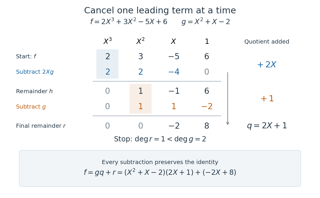
The polynomial degree bound makes this decomposition useful: it replaces a potentially long polynomial with a short polynomial remainder whenever multiples of

g

can be discarded. At any root of a polynomial of

g

, those multiples vanish under polynomial evaluation. Repeated polynomial division also drives the Euclidean algorithm for finding a greatest common divisor of polynomials.

The coefficient setting matters. Over a commutative ring, the same existence and uniqueness hold when the divisor's leading coefficient is a unit in a ring. A monic polynomial therefore works over the integers, even though they do not form a field; monic polynomial division over a ring explains why zero divisors cause no difficulty in that case.^[ref]

A nonzero divisor alone is insufficient over the integers. Dividing

X

2 X + 1

with an integer polynomial quotient and a constant polynomial remainder would require

1 = 2 c

for an integer

c

, which is impossible. Over the rational numbers the division instead gives

X = (2 X + 1) \frac{1}{2} - \frac{1}{2} .

(6)

The obstruction is the nonunit leading coefficient

2

. This example separates existence from uniqueness: over an integral domain, the polynomial degree argument still makes any admissible pair unique, if it exists.

Prescribing a factor by elliptic-curve tripling 2026-10-31

Let

N = pq

with primes

p \equiv 1 (mod 12)

and

q \equiv 5 (mod 12)

. quadratic reciprocity makes three a square modulo

p

; choose

r^{2} = 3

and impose

a = - 3 + 2 r (mod p)

a = 1 (mod q)

by the Chinese remainder theorem. The curve has good reduction at both primes. Indeed its discriminant is

- 16 a^{2} (4 a + 27)

; the first condition could make a factor vanish only at

p = 3

or 11, while the second gives

a (4 a + 27) = 31

and the given residue class excludes

q = 31

Doubling

P

gives

x (2 P) - 1 = (a^{2} + 6 a - 3) /4

. This vanishes modulo

p

and equals one modulo

q

. Modulo

p

one also has

y (2 P) = - 1

, so

2 P = - P

and

3 P

is the identity. Modulo

q

the addition is finite. Thus computing

3 P

modulo

N

encounters a denominator whose greatest common divisor with

N

is exactly

p

, revealing the factor. The numerator difference is minus two modulo

p

, so the failed inverse cannot be cancelled. This is a construction of successful elliptic curve method data from prescribed local group behavior.

Prime number Created 2026-09-24 Updated 2026-10-13

A prime number is a positive integer

p > 1

whose only positive divisors are

1

and

p

. The first ten prime numbers are

2, 3, 5, 7, 11, 13, 17, 19, 23, 29

. In contrast,

12 = 3 \cdot 4

is a composite number because it has a positive divisor strictly between one and itself. The integer one is neither a prime number nor a composite number: the lower bound

p > 1

is part of the definition. Equivalently, the divisor function satisfies

τ (p) = 2

for a prime number, whereas

τ (1) = 1

and

τ (n) \geq 3

for every composite number

n

Prime numbers are the building blocks of positive integers under multiplication. The fundamental theorem of arithmetic says that every integer greater than one is a product of prime numbers, with a unique collection of factors when their order is ignored. For example,

12 = 2 \cdot 2 \cdot 3

and

18 = 2 \cdot 3 \cdot 3

. Their common factors reveal the greatest common divisor

6

, and the combined maximum powers reveal the least common multiple

36

. A complicated divisibility question becomes a comparison of prime exponents.

There is also a useful finite test. If a composite number

n

equals

ab

with

1 < a \leq b

, then

a^{2} \leq n

. Therefore some prime factor is at most

n

, and trial division only needs to check prime numbers up to that square root. For

97

, checking

2, 3, 5, 7

suffices; none divides

97

, so it is a prime number. For

91

, the same test finds

7

, giving

91 = 7 \cdot 13

. To find many prime numbers together, the sieve of Eratosthenes reuses the work by marking multiples.

The division with remainder calculations for

97

make the test explicit:

97 = 2 \cdot 48 + 1 = 3 \cdot 32 + 1 = 5 \cdot 19 + 2 = 7 \cdot 13 + 6.

Since

9^{2} < 97 < 1 0^{2}

, these are all the prime numbers at most its square root, and every remainder is nonzero. Thus the calculation certifies a prime number, without testing the integers

8, 9, 10, \dots, 96

individually. In contrast,

91 = 7 \cdot 13 + 0

gives a prime factor and proves that

91

is a composite number.

Prime omega function Created 2026-09-28 Updated 2026-10-13

The prime omega function

ω (n)

counts the distinct prime factors of a positive integer

n

, so it is the cardinality of the prime support of an integer

P (n)

. For a prime factorization with distinct prime numbers

p_{1}, \dots, p_{r}

and positive exponents,

n = p_{1}^{a_{1}} \dots p_{r}^{a_{r}} ⟹ ω (n) = r = \sum_{p ∣ n} 1.

n = 1

there are no prime factors, so the empty sum gives

ω (1) = 0

. The total number of prime factors instead gives

Ω (n) = \sum_{i} a_{i}

. ^[ref]

For

72 = 2^{3} \cdot 3^{2}

, the prime support of an integer is

{2, 3}

and

ω (72) = 2

. The comparison examples give

ω (30) = 3

ω (32) = 1

and

ω (36) = 2

. Raising an existing prime factor to a higher power does not affect the prime omega function:

ω (p^{k}) = 1

for a prime number

p

and

k \geq 1

. Thus the prime omega function is a strongly additive arithmetic function, with

ω (ab) = ω (a) + ω (b) if g cd (a, b) = 1.

The reason is that coprime integers have disjoint prime supports of an integer. For arbitrary positive integers, their prime support of an integer combines by set union, and the shared prime factors are exactly those of the greatest common divisor. Counting this set union gives the more general identity

ω (ab) = ω (a) + ω (b) - ω (g cd (a, b)) .

(3)

For

a = 12

b = 18

, both prime supports of an integer are

{2, 3}

and

g cd (a, b) = 6

, so

ω (216) = 2 + 2 - 2 = 2

. In particular

ω (4) = 1 \neq = 2 = ω (2) + ω (2)

: the prime omega function is not a completely additive arithmetic function.

The prime omega function is useful for counting choices involving distinct prime factors. Every squarefree divisor of

n

chooses a subset of its prime support of an integer, so there are

2^{ω (n)}

squarefree divisors. For

72

, this gives

2^{2} = 4

, namely

1, 2, 3, 6

. Also

ω (rad (n)) = ω (n)

, because the radical of an integer keeps exactly that prime support of an integer. The total number of prime factors records what this count discards, and the two counts agree exactly on squarefree integers.

Primitive Diophantine solution 2026-10-20

A primitive Diophantine solution is an integer tuple satisfying the equation whose coordinates have greatest common divisor one. For homogeneous equations, this removes common integer scale factors.

Primitive lattice element Created 2026-10-06 Updated 2026-10-14

A nonzero element of a free abelian group is primitive when it is part of an integral basis, equivalently when some homomorphism to

Z

takes it to one. Its coordinates have greatest common divisor one. This lattice meaning differs from a primitive homology class in the coalgebra sense.

Primitive Pythagorean triple 2026-10-20

A Pythagorean triple

(a, b, c)

whose coordinates have greatest common divisor 1. Its two legs have opposite integer parity, and every Pythagorean triple is a unique positive integer multiple of a primitive Pythagorean triple up to the ordering of its legs.