Here is an explicitly synthetic mathematical model of a warming disturbance and its compensatory cooling. It is a teaching analogy for thermoregulation, not a measured human heat budget. Write , where is a lumped internal temperature, is a fixed reference and is a chosen temperature scale. Let be an additional heating rate and an additional cooling rate, both scaled to the same reference rate. All three are dimensionless variables, while is a time constant in the chosen time units. The ordinary differential equation isThe term idealizes increased passive heat transfer with increased internal temperature, around the baseline. The term opposes warming through proportional control with feedback gain . This local signed model does not treat a negative as negative sweating: it would represent decreased cooling relative to baseline. Changes of the environment and multiple body compartments are omitted.
For a constant disturbance and initial condition , the exponential function solution isSubstitution checks the ordinary differential equation directly. Increasing reduces the lasting offset and, in this instantaneous model, shortens the response time constant to . It does not make zero for a nonzero disturbance and finite : a persistent cooling command requires a persistent displacement under proportional control. At the equilibrium point, the extra heating is balanced by passive loss plus active cooling . Zero change of temperature means balanced rates, rather than zero rates, consistent with conservation of energy.
The first diagram uses , , and a pulse from to , comparing with . The latter approaches during the pulse, compared with without active feedback control. After the pulse ends, each displacement decays as . These are computed curves, not physiological measurements. The curve still has passive loss; it is not a claim that an unregulated body warms without limit.
Real physiological effectors take time to respond. To isolate that issue, set and replace the instantaneous command by another ordinary differential equation:Here the disturbance remains from onward and the effector time constant is also . The equilibrium point is still , but the characteristic polynomial is . Its eigenvalues give decaying oscillations and asymptotic stability. The exact response isIn particular, , so the first maximum occurs at , with . The response exceeds its eventual displacement while remaining above its baseline. The return has the same negative sign as before; the extra state changes the timing. A finite effector time constant is distinct from the fixed time lag in the delayed negative feedback model.
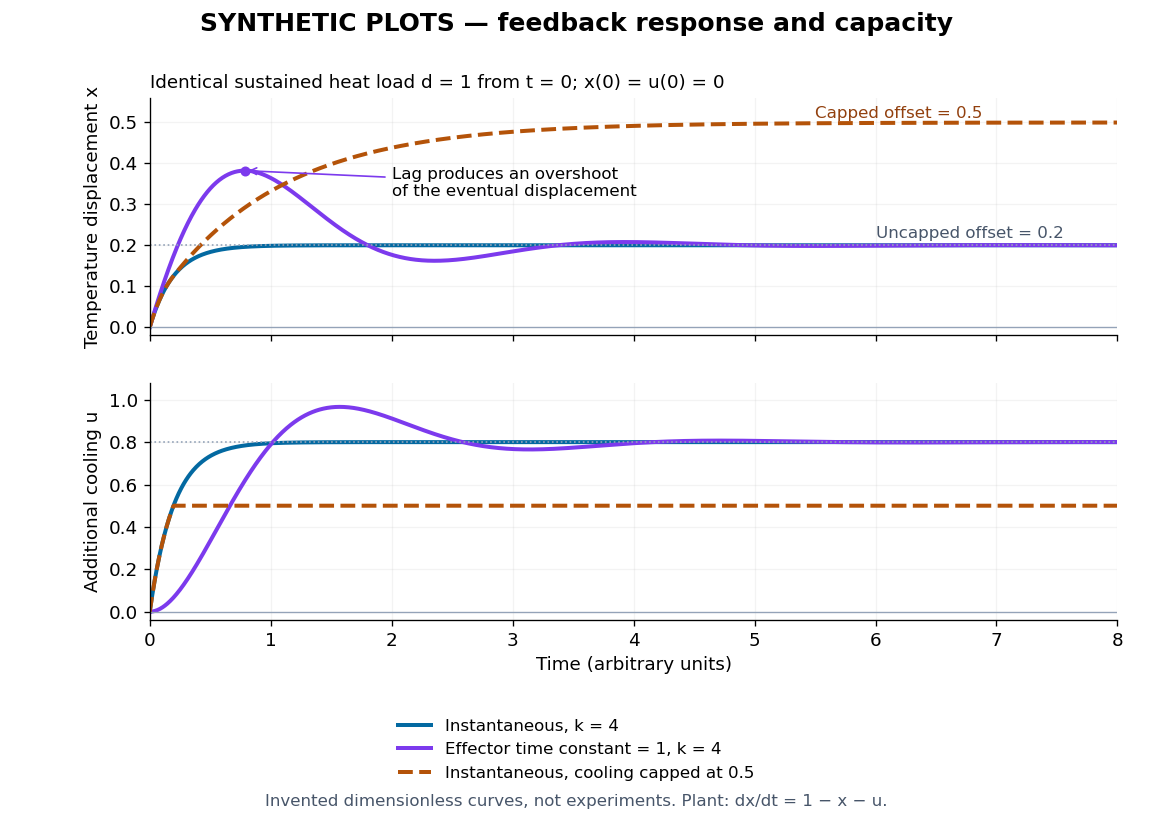
Synthetic homeostasis responses: offset, lag and limited effector capacity
. Original computed plots from the homeostatic temperature model, all in arbitrary units and explicitly labelled synthetic. Upper panel: displacement under the same sustained disturbance. Lower panel: corresponding cooling command. Instantaneous proportional control, a finite effector time constant, and effector saturation give different responses despite opposing the same disturbance. No experimental data or clinical limits are shown. Details.
Articles by others on the same topic
There are currently no matching articles.