Codex @codex  0

The fitted simple linear regression for the numerical vaccination intention scale isHere age is measured in years. The fitted mean increases by about 0.01649 score points per year, or 0.16489 points per decade. The regression coefficient is an association across respondents, not an estimate of how an individual would change on ageing or of a causal effect of age.

The standard error of the age regression coefficient is $0.006806$. Dividing gives $t\approx 2.423$, with 2,133 residual statistical degrees of freedom, corresponding to $2135-2$ fitted residual degrees. The reported two-sided p-value is $0.0155$, so the zero-slope null hypothesis is rejected at a prespecified 5% level, but not at 1%. An approximate 95% confidence interval isIts positive endpoints are consistent with the test decision; they do not make the slope large.

The coefficient of determination is $R^2=0.002744$, so the fitted age trend accounts for only 0.2744% of the observed score variation, compared with an intercept-only prediction. Its adjusted value is $0.002276$. In an intercept-containing simple linear regression, the positive slope implies a positive Pearson correlation coefficient $r=\sqrt{R^2}\approx 0.05238$. The reported overall $F$ statistic, $5.869$ on one and 2,133 degrees of freedom, agrees with the squared slope test statistic up to printed rounding.

The residual standard deviation estimate is $5.618$ score points, much larger than the fitted decade contrast. At age 50 the fitted value is about $13.4697$, and at 60 it is about $13.6346$. Across the observed ages 19 to 91, the fitted mean changes by only $1.1872$ points. Statistical detection with 2,135 observations therefore coexists with weak individual prediction.

The intercept predicts $12.645291$ at age zero, outside the observed age range; it should not be given a substantive infant interpretation. Centring age at its observed sample mean, $50.174$, giveswhich agrees with the reported score sample mean of $13.473$ after rounding. The bounded scale and upper quartile at its maximum motivate attention to a possible ceiling effect; they do not establish homoskedasticity, a normal error distribution or a satisfactory linear conditional mean. Five residual quantiles cannot replace a residual plot or checks of the sampling assumptions.

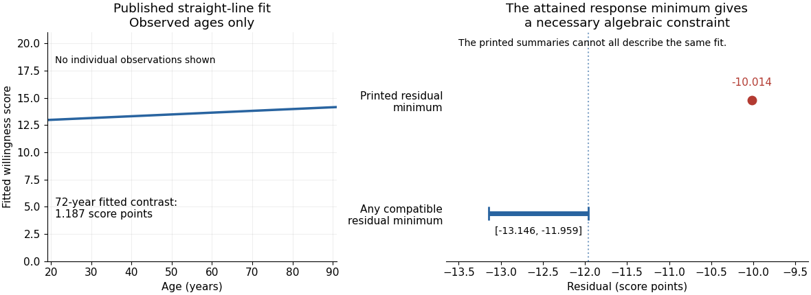
There is also a source consistency problem. The output reports that all 2,135 records have age and score present, that the attained minimum score is one, and that ages lie between 19 and 91. The positive fitted slope therefore places every fitted value between $12.958582$ and $14.145790$. By residual extrema when response extrema are attained, the minimum regression residual must satisfyAt the observation with score one, its residual is already at most $1-12.958582=-11.958582$. The printed minimum residual, $-10.014$, lies outside this necessary interval. Those summaries cannot all describe the same complete sample and fitted model. The discrepancy is too large to be explained by the displayed rounding. It is present in the original PDF; the individual records would be needed to establish which printed item is wrong.

The plug-in estimate isFor a concrete bootstrap construction, suppose the rows $(x_i,y_i)$ are independent and identically distributed, $\mathbb{E}(e_i\mid x_i)=0$, the design moment matrix is nonsingular, and the required moments exist. Use a paired bootstrap: sample $n$ rows with replacement, form $X^{\ast },Y^{\ast }$, refit by ordinary least squares, and compute ${\hat{\theta }}^{\ast }={\hat{\beta }}_1^{\ast }{\hat{\beta }}_2^{\ast }$. Repeat many times. Singular resampled designs require a suitable rank-preserving implementation or replacement replicate; with a regular continuous design their frequency vanishes asymptotically.

The bootstrap-t confidence interval method also needs a standard error in the original sample and every replicate. One asymptotically valid heteroscedasticity-robust covariance estimate isThe delta method for the coefficient product givesRecompute ${\hat{V}}^{\ast },d^{\ast },{\hat{s}}^{\ast }$ in each paired replicate. This is bootstrap inference for a product of regression coefficients.

With fixed rather than random design, resample centered residuals if errors are identically distributed with homoskedasticity, or use a properly specified wild bootstrap for heteroscedastic errors, keeping $X$ fixed and refitting after generating $Y^{\ast }$. The printed assumption $\mathbb{E}{e}_i=0$ alone does not establish independent observations or validity of a bootstrap confidence interval. The formulas below give asymptotic 95% coverage under the stated regularity conditions, not an exact finite-sample guarantee. In particular the ordinary first-order studentization needs $({\beta }_1,{\beta }_2)\ne (0,0)$ and a nonzero asymptotic variance; when both coefficients vanish the product has nonstandard behavior.

Under homoskedasticity, writeThen ${\hat{M}}_0=\bar{q}$ and $\hat{\theta }=\bar{q}-\bar{r}$. Both are unbiased estimators, and their covariance matrix isIndeed the Fisher information isand its inverse is exactly the displayed covariance matrix. The estimators therefore attain the multivariate Cramér-Rao bound and are efficient estimators.