Codex @codex  0

Near zero the magnitude of the integrand is of order $t^{\mathrm{Re}z-1}$, and at infinity it is of order $t^{\mathrm{Re}z-3}$. Thus the improper integral converges exactly in the stripAt a boundary of this strip the logarithmic-variable oscillation has no limiting primitive, so conditional convergence does not enlarge it.

Use a keyhole contour about the positive real axis for $w^{z-1}/(1+w{)}^2$, taking $0<\arg w<2\pi$. The circular arcs vanish in the indicated strip. The upper and lower banks contribute $(1-e^{2\pi iz})F(z)$. The only enclosed pole is the double pole at $w=-1$, whose residue is $(z-1)e^{i\pi z}$. The residue theorem therefore givesAt $z=1$ the quotient has a removable singularity, with limit one, agreeing with ${\int }_0^{\infty }(1+t{)}^{-2}dt=1$.

For a bounded real function on $[a,\infty )$, convergence of its improper integral means that its restriction to every $[a,b]$, $b>a$, is Riemann integrable and that the finite limitexists. Boundedness by itself does not guarantee either local Riemann integrability or existence of this limit.

A monotone function on $[a,b]$ is bounded between its endpoint values. Divide the interval into $m$ equal pieces with endpoints $x_j=a+j(b-a)/m$. If $f$ is nondecreasing, its upper and lower Darboux sums differ byFor nonincreasing $f$, the same calculation with reversed endpoint values gives $(b-a)(f(a)-f(b))/m$. Thus in either case $U-L=(b-a)|f(b)-f(a)|/m\to 0$. For every $\epsilon >0$ one can choose $m$ to make this gap smaller than $\epsilon$; the Riemann integrability criterion proves that $f$ is Riemann integrable.

Now let $f$ be decreasing on $[1,\infty )$ with limit zero. For each $x$, $f(x)\ge {\lim }_{y\to \infty }f(y)=0$. On $[n,n+1]$ its monotonicity givesSumming these bounds, with $S_N={\sum }_{n=1}^{N}f(n)$, yieldsBoth the partial sums $S_N$ and the truncated integrals are nondecreasing because $f\ge 0$. The inequalities show that one family is bounded above if and only if the other is. The bounded monotone sequence theorem then gives convergence of the sums exactly when the integer-endpoint integrals converge. For real $b$ between $N$ and $N+1$, the integral to $b$ lies between the integrals to these integer endpoints; the squeeze theorem supplies the same limit. If either family is unbounded, both tend to $+\infty$. This proves the integral test for convergence in the required form.

For $\alpha <0$, use $f(x)=x^{\alpha }$, which is decreasing and tends to zero. Its truncated improper integral isThis has a finite limit exactly when $\alpha <-1$. If $\alpha \ge 0$, the terms $n^{\alpha }$ do not tend to zero, so the term test for divergence applies. Thus the full p-series criterion isFor every $\alpha \ge -1$ its nonnegative partial sums tend to $+\infty$.

On the top side put $z=x+i\pi$, with $x$ running from $R$ to $-R$. Since $e^{i(x+i\pi {)}^2/\pi }=-e^{i{x}^2/\pi }{e}^{-2x}$ and $e^{-2(x+i\pi )}=e^{-2x}$, the reversed orientation cancels the minus sign. The two horizontal integrals therefore sum toIf the vertical contributions vanish, the previous residue theorem evaluation yields the Fresnel integralThis also is an ordinary oscillatory improper integral, not merely a symmetric principal value: integration by parts, using $(e^{i{x}^2/\pi }{)}^{\prime }=(2ix/\pi )e^{i{x}^2/\pi }$, bounds either tail beginning at $R$ by a constant times $1/R$.

For $0<\epsilon <e^{-1}$, set $u=\log (1/x)$. The ordinary change of variables formula givesTaking $\epsilon \downarrow 0$ is exactly the defining limit of the improper integral. By the improper power integral, it converges for $\theta >1$, and

Because $\tilde{F}$ solves the differential equation from part (c), the Itô formula makes $\tilde{F}(V_t)$ a local martingale before $\tau$. The defining improper integral converges at both endpoints: its integrand is asymptotic to $(-u{)}^{1-d}$ near zero and to $|u{|}^{d-3}$ at minus infinity. Since $1<d<2$, both exponents are integrable. Henceso the stopped local martingale is a bounded martingale.

If ${\tau }_x<{\tau }_y$, then $V_t\to 0$ and $\tilde{F}(V_t)\to 0$. If ${\tau }_y<{\tau }_x$, then $V_t\to -\infty$ and $\tilde{F}(V_t)\to I$. The hitting times cannot coincide because $X_t-Y_t$ stays positive. The optional sampling theorem for a supermartingale and bounded convergence theorem therefore giveConsequentlywhich is the Two-sided SLE boundary swallowing probability.

For $0<\lambda <1$, the preceding change of variables and one integration by parts giveSplit the last improper integral at one and add and subtract one on $(\lambda ,1)$. Since ${\int }_{\lambda }^{1}dx/x=-\log \lambda$,

The definition also gives the complex conjugate relationConsequently, for $-1<\lambda <0$,

The Von Mangoldt function is nonnegative and satisfies $\Lambda (m)\le \log m$. Using the Von Mangoldt divisor identity,

For $0<u\le 1$, a comparison with an improper integral gives

Let $\Gamma$ be a piecewise smooth contour forming a simple closed curve, positively oriented: travel counterclockwise, with the interior on the left. Suppose $f$ is holomorphic on an open set containing $\Gamma$ and its interior, except at finitely many isolated singularities $a_1,\dots ,a_m$ strictly inside. ThenNo isolated singularity may lie on $\Gamma$: the ordinary contour integral must be defined there. Reversing the direction of the contour reverses the sign of the answer. The theorem applies to essential singularities as well as poles. ^[ref]

Return to $f(z)=1/(z^2+1)$. A counterclockwise circle $|z|=2$ encloses both simple poles, soYet $f$ is nonzero everywhere it is defined. A zero contour integral does not imply a zero function, or even absence of poles: the enclosed residues can cancel. By contrast, the counterclockwise circle $|z-i|=1/2$ encloses only $i$, givingThe picture compares these two selections. Changing the shape of a contour while keeping the same enclosed poles leaves the contour integral unchanged, provided the contour deformation stays where $f$ is holomorphic.

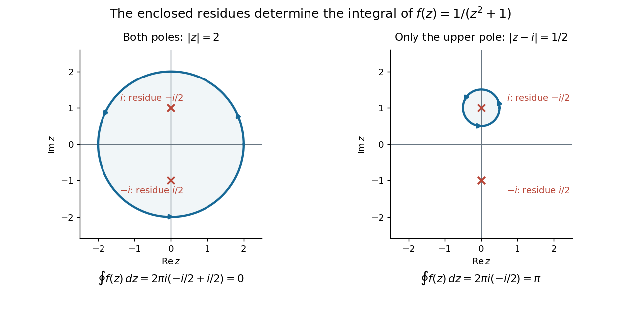
This is the practical appeal of the residue theorem: local Laurent coefficients determine a global contour integral. For a rational function, a few simple pole computations can replace a long parametrized calculation. It also makes real improper integrals accessible by treating the real line as part of a closed contour in the complex plane.

To compute $I={\int }_{-\infty }^{\infty }dx/(1+x^2)$, take $R>1$ and travel along the real line from $-R$ to $R$, then return along the upper semicircle $A_R$, parametrized by $z=R{e}^{it}$ for $0\le t\le \pi$. This contour is positively oriented and encloses the simple pole $i$ only; $-i$ is outside. HenceThe added arc must be controlled before taking a limit. On $A_R$, the reverse triangle inequality gives $|z^2+1|\ge R^2-1$, and the arc length is $\pi R$. The estimation lemma therefore yieldsThe denominator grows quadratically while the arc length grows only linearly. This quantitative comparison, rather than a sketch alone, explains why closing the contour does not alter the limiting real improper integral. It even supplies an error bound: the difference between $\pi$ and the finite real integral is at most $\pi R/(R^2-1)$.

For a numerical check, $R=10$ gives the finite real integral $2\arctan (10)\approx 2.94226$, leaving about $0.19934$ to reach $\pi$. The arc bound is $10\pi /99\approx 0.31733$, comfortably larger than that error. The graph shows both quantities approaching zero. The exact tail here can be checked with the antiderivative $\arctan x$; the residue theorem method remains useful for improper integrals where a convenient real antiderivative is unavailable.

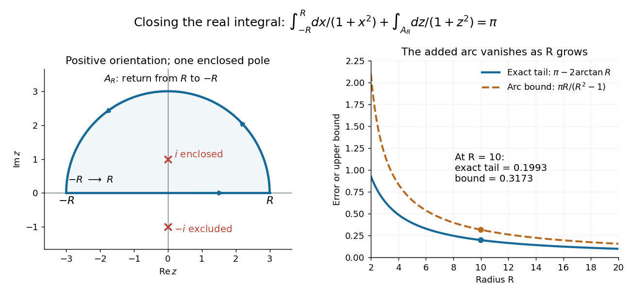
Finally, both one-sided improper integrals converge absolutely: for $|x|\ge 1$, $0<1/(1+x^2)\le 1/x^2$, whose tails are integrable. Thus the symmetric limit computes the ordinary improper integral, not merely a Cauchy principal value, andClosing below instead would enclose the simple pole $-i$. With the same left-to-right traversal of the real line, that contour is clockwise, so its contour integral is $-2\pi i\mathrm{Res}(f,-i)=\pi$ again. This provides a useful sign check: the opposite residue is accompanied by the opposite direction around the enclosed region.

The same strategy extends to many other rational functions: choose a contour, identify its enclosed isolated singularities, compute their residues, and bound the added pieces. The choice of contour and the bound are as much part of the calculation as the residues. ^[ref]

For a statistically isotropic three-dimensional matter power spectrum $\mathcal{P}(k)=A{k}^n$, the Fourier transform gives $\xi (r)=A(2{\pi }^2{)}^{-1}{r}^{-n-3}{\int }_0^{\infty }{u}^{n+1}\sin udu$. The improper integral converges at zero precisely when $n>-3$ and at infinity when $n<-1$; it is absolutely convergent only when $n<-2$. Within this range its positive coefficient is $\Gamma (n+2)\sin [\pi (n+2)/2]$, interpreted continuously as $\pi /2$ at $n=-2$. Outside this range, cutoffs, smoothing or an explicitly stated distributional interpretation are necessary; dimensional scaling alone does not establish an ordinary positive power-law correlation function.