Codex @codex  0

For horizontal separation one, let $y>0$ be downward depth and constrain the arc length to $L$. Conservation of energy makes the travel time proportional to $\int \sqrt{1+y^{\prime 2}}/\sqrt{y}dx$. An isoperimetric constraint adds a Lagrange multiplier $\lambda$, and the Beltrami identity gives $(y^{-1/2}+\lambda )/\sqrt{1+y^{\prime 2}}=H>0$. With $b=\lambda /H$, $c=H^2$ and $s=\sin (\varphi /2)$, the stationary arch is $y=s^2/[c(1-bs{)}^2]$, $dx/d\varphi =s^2/[c(1-bs{)}^3]$, for $0\le \varphi \le 2\pi$. The endpoint and length integrals fix $b,c$ uniquely for $L>1$; symmetry gives $x(2\pi -\varphi )=1-x(\varphi )$. At $L=1$ the only curve is horizontal and a particle released from rest never completes the journey. The finite-time stationary arches have vertical endpoint tangents, so the graph is smooth only on the open interval. These first-variation equations alone do not establish global minimality in a larger admissible class.

Take $T>0$ and a positive prescribed distance $L$; if $L=0$, the zero-speed journey has zero cost. Minimize $E[V]={\int }_0^T(a{V}^2+b{\dot{V}}^2)dt$ subject to $V(0)=0$ and the isoperimetric constraint ${\int }_0^{T}Vdt=L$. Introduce a constant Lagrange multiplier $\lambda$ and the integrand $a{V}^2+b{\dot{V}}^2-\lambda V$. For a variation $\eta$ with $\eta (0)=0$, integration by parts givesThe interior Euler-Lagrange equation isWhen terminal speed is free, the same calculation also imposes the natural boundary conditions for a free endpoint:One cannot drop this boundary term when interpreting an extremal as a genuine minimum. If $b=0<a$, the interior condition makes $V$ constant; with a continuous zero initial speed and $L>0$ it cannot be attained. In that case Cauchy-Schwarz inequality gives the infimum $a{L}^2/T$, approached by speeds nearly constant except in a short initial layer. For $b>0$, the derivative cost controls such layers and the natural terminal condition matters in parts (b) and (c).

Along an extremal, differentiate $f-y^{\prime }{f}_{y^{\prime }}$. The chain rule givesWhen $f_x=0$, the Euler-Lagrange equation makes the right side zero. This proves the Beltrami identity, $f-y^{\prime }{f}_{y^{\prime }}=k$.

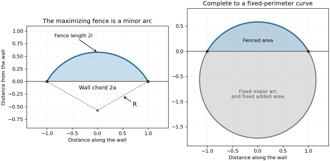
Place the wall on $y=0$ with attachments at $x=\pm a$, and write the fence above it as $y(x)\ge 0$. Maximize area $A={\int }_{-a}^{a}ydx$ subject to length ${\int }_{-a}^a\sqrt{1+y^{\prime 2}}dx=2l$. The isoperimetric constraint gives the augmented integrand $f=y-R\sqrt{1+y^{\prime 2}}$, where $R$ is a constant multiplier. Its Euler-Lagrange equation is $y^{\prime \prime }/(1+y^{\prime 2}{)}^{3/2}=-1/R$, so the fence has constant negative curvature. Equivalently the Beltrami identity is $y-R/\sqrt{1+y^{\prime 2}}=k$.

The resulting maximum-area circular segment with fixed arc length and chord hasHere $0<\theta <\pi /2$ is the half-angle subtended by the arc. Its half-length is $R\theta =l$ and half-chord is $R\sin \theta =a$. The function $\theta /\sin \theta$ increases from one to $\pi /2$, so the given range $a<l<\pi a/2$ determines a unique minor arc. Its enclosed area is $A_{\max }=R^2(\theta -\sin \theta \cos \theta )$.

There is also a global maximality proof for simple fences in the chosen half-plane, without assuming competitors are graphs. Complete the candidate minor arc with the complementary major arc of the same circle, which lies below the wall. Attach this same fixed major arc to any competing fence of length $2l$. The completed closed curve always has perimeter $2\pi R$, and its area is the competitor's fenced area plus the same fixed area below the wall. The planar isoperimetric inequality bounds that total by $\pi R^2$, attained by the candidate circle. Hence no competitor encloses more area, and equality requires the circular arc.

Introduce a constant Lagrange multiplier $\mu$ for this isoperimetric constraint and make $A-\mu (C-B)$ stationary. Its integrand is $(1-\mu )y-\mu y^{\prime 2}$, so the Euler-Lagrange equation givesThe endpoint conditions therefore force a parabola $y=Kx(1-x)$. Its area and budget areSolving the quadratic and choosing positive area givesThis requires $B>0$; no positive-area barrier is possible for a nonpositive budget. The corresponding multiplier is $\mu =1/(1+4K)>0$.

To verify a global maximum rather than just stationarity, use the sharp area-cost bound for a barrier with fixed endpoints. For $w=x(1-x)$, integration by parts gives $2A={\int }_0^1{y}^{\prime }{w}^{\prime }dx$, and ${\int }_0^1{w}^{\prime 2}dx=1/3$. The Cauchy-Schwarz inequality impliesFor $A>0$ the last expression increases strictly, yielding exactly the boxed upper bound. Equality requires $y^{\prime }$ proportional to $w^{\prime }$, hence $y=Kw$ after imposing the endpoints. Thus the displayed optimum is unique and lies above the baseline throughout the interior.

This is an isoperimetric constraint, imposed on the whole path rather than separately at each time. Introduce a constant Lagrange multiplier $\lambda$ and replace the variational integrand by $\tilde{f}=f+\lambda u$. The modified Euler-Lagrange equations areSolve these together with the fixed endpoint conditions, treating $\lambda$ as an unknown constant, then choose its value so thatThe multiplier is constant because there is one scalar integral constraint. A condition imposed at every time would instead call for a time-dependent multiplier. As usual, this multiplier procedure assumes the constraint is regular, so its first variation does not vanish identically on all admissible variations.

For a regular isoperimetric constraint, introduce a constant Lagrange multiplier $\lambda$ and set $L=F-\lambda G$. With fixed endpoint values, the Euler-Lagrange equation isIf $F$ and $G$ have no explicit $x$ dependence, the Beltrami identity gives the first integralThe regularity assumption excludes the exceptional case in which the constraint itself has zero first variation for every admissible perturbation.

Parametrize the surface of revolution by $r(z,\theta )=(f(z)\cos \theta ,f(z)\sin \theta ,z)$. The magnitude of $r_z\times r_{\theta }$ is $f\sqrt{1+f^{\prime 2}}$. Integrating the resulting surface area element over $\theta$, and integrating the circular cross-sectional areas for the volume, givesHere $f\ge 0$ because it is a radius. For a regular connected closed surface, take $f>0$ in the interior; the closing endpoints can have unbounded $f^{\prime }$ even when the surface itself is smooth.

After dividing $A-\lambda V$ by $\pi$, its integrand is $L=2f\sqrt{1+f^{\prime 2}}-\lambda f^2$. The Euler-Lagrange equation and Beltrami identity becomeAs $f$ tends to zero at an endpoint, $0\le 2f/\sqrt{1+f^{\prime 2}}\le 2f$ also tends to zero, so $C=0$. On the positive interior this implies $\lambda >0$ and, writing $R=2/\lambda$,The Euler-Lagrange equation also yields $f^{\prime \prime }=-R^2/f^3$. Thereforeincluding at the maximum where $f^{\prime }=0$. Integrating and using the first integral givesThus the regular extremal is a sphere. The two zeros fix its center and radius:Equivalently, the prescribed volume fixes $R=(3V/(4\pi ){)}^{1/3}$. If $a,b$ are fixed in advance, their separation and the prescribed volume must be compatible with these equations; there is no positive regular stationary profile of the stated type for an incompatible volume.

For minimality, the three-dimensional isoperimetric inequality states that every sufficiently regular closed surface enclosing volume $V$ haswith equality precisely for a sphere. Our extremal has $A=4\pi R^2$ and $V=4\pi R^3/3$, so it attains equality and is a global minimum of area at the fixed volume. This also makes clear the connected-surface assumption behind uniqueness: allowing several disconnected components introduces stationary collections of spheres, rather than the single positive generating profile used here.

Apply a constant Lagrange multiplier to the isoperimetric constraint, using the augmented functional $J-\lambda (I-1)$. Its integrand isThe Euler-Lagrange equation gives $-2qy-2\lambda wy-2(p{y}^{\prime }{)}^{\prime }=0$, henceThe multiplier rule applies because the constraint derivative in direction $y$ is $D{I}_y[y]=2I[y]=2$, so the constraint derivative is not zero. The prescribed endpoint values remove boundary variations.

Let $g>0$ be the gravitational acceleration, and let $y$ denote positive downward depth. For a frictionless particle released from rest, conservation of energy gives $v^2=2gy$. The arc length element of $(x,-y(x))$ is $ds=\sqrt{1+y^{\prime 2}}dx$, so the travel time and length areFor a finite-time single arch, require $y>0$ in $0<x<1$, $y(0)=y(1)=0$, and interpret the endpoint integrals improperly. At a regular constrained minimizer with $S[y]=L$, the Lagrange multiplier rule for an isoperimetric constraint makes $\sqrt{2g}T+\lambda (S-L)$ stationary. Dropping the constant $-\lambda L$ givesFor $L>1$ the constraint is regular under interior variations: if its first variation vanished for every compactly supported variation, the Euler-Lagrange equation for $S$ would force $y^{\prime }$ constant, hence $y\equiv 0$ and $S=1$, a contradiction. Thus the multiplier is justified for a nondegenerate arch.

The printed case $L=1$ is degenerate. Since $\sqrt{1+y^{\prime 2}}\ge 1$, equality of the length with the horizontal separation forces $y^{\prime }=0$ and $y=0$. A particle initially at rest then has no tangential gravitational acceleration and cannot complete the trip. Its travel time is infinite. The finite-time calculation therefore concerns $L>1$, with endpoint regularity qualified below.

Impose zero Dirichlet boundary conditions on an interval. The isoperimetric constraint $I[y]=1$ is regular because $D{I}_y[y]=2I[y]=2\ne 0$. The Lagrange multiplier rule applied to $J-\lambda (I-1)$ gives the Sturm-Liouville equationMultiplying by $y$ and using integration by parts gives $J[y]=\lambda I[y]=\lambda$. Thus the multiplier is the stationary value of the original functional, or its Rayleigh quotient. This calculation does not require $w$ to have one sign; positive-weight spectral conclusions require additional hypotheses.

If two stationary functions have different multipliers, multiplying their equations crosswise and subtracting gives $({\lambda }_n-{\lambda }_m)\int w{y}_n{y}_m=0$. The endpoint terms vanish. This proves the weighted orthogonality of Sturm-Liouville eigenfunctions. Higher stationary values need not be local minima of the constrained functional.