Codex @codex  0

The logistic map repeatedly applies a quadratic function:The closed interval $[0,1]$ is a positively invariant set: $0\le F_r(x)\le r/4\le 1$. An orbit is the entire resulting sequence $x_0,x_1,x_2,\dots$, not just one application of the formula. For example, with $r=2$ and $x_0=0.2$, the first states are $0.2,0.32,0.4352,0.49160192,\dots$, approaching the fixed point $1/2$.

As a simple model of population dynamics, $x_n$ is a scaled abundance in generation $n$. When abundance is small, $x_{n+1}/x_n=r(1-x_n)$ is close to $r$; increasing abundance reduces this per-capita multiplier. The falling side of the quadratic function represents sufficiently severe crowding reducing the next generation. The scale $x=1$ is not generally the carrying capacity: the positive fixed point is $1-1/r$. The logistic map is a discrete-generation model; the continuous-time logistic growth equation has a different evolution rule and does not produce its period-doubling cascade.

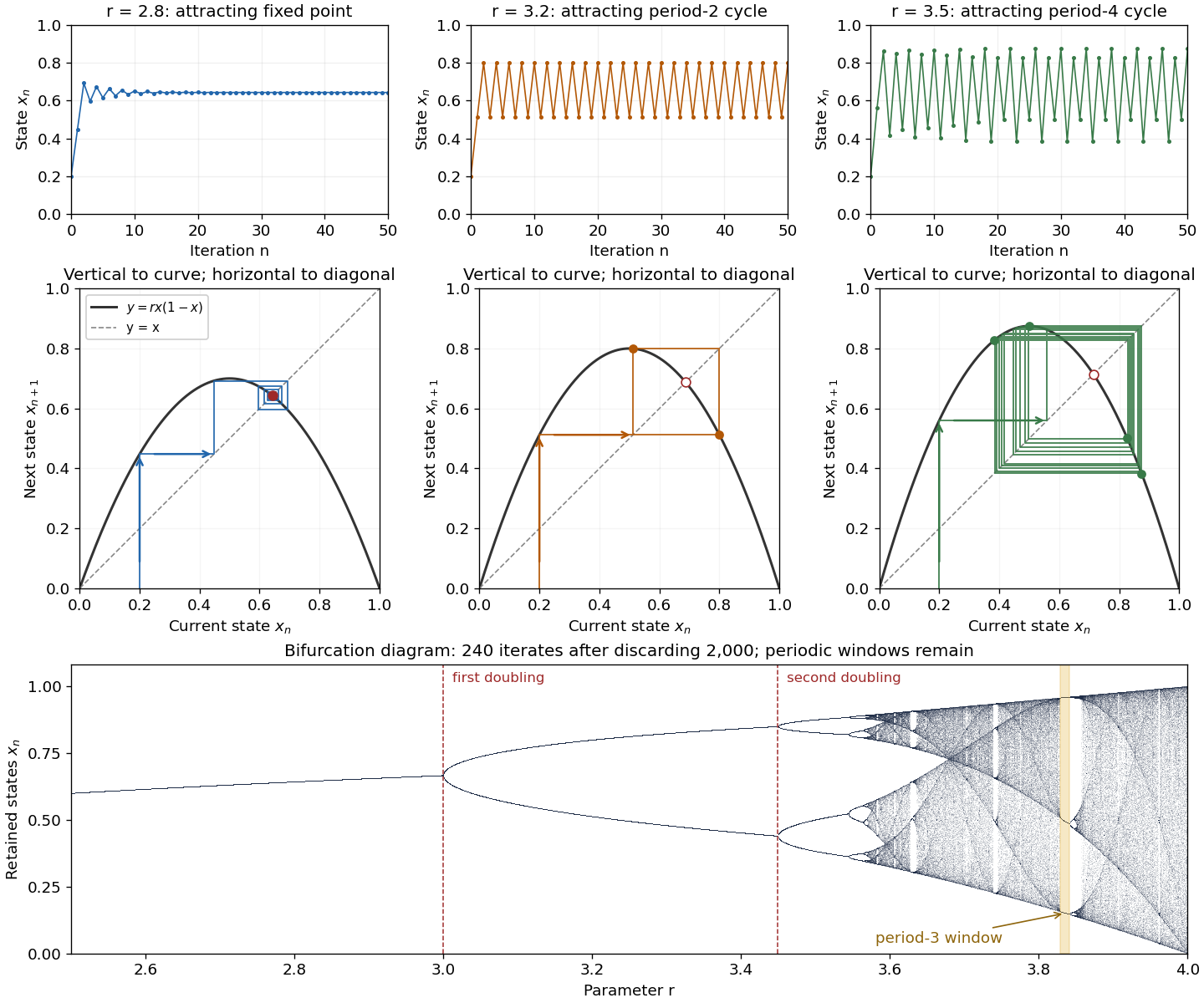
The practical question is how abundance behaves after the initial adjustment: does it settle, alternate, or continue varying? The same formula permits all these possibilities. The following figure shows three orbits, their cobweb plots, and a bifurcation diagram. In a cobweb plot, moving vertically to $y=F_r(x)$ calculates the next state, and moving horizontally to $y=x$ makes that value the input for the next step.

The fixed points solve $F_r(x)=x$:The second fixed point is in $[0,1]$ for $r\ge 1$ and coincides with zero at $r=1$. The derivative is $F_r^{\prime }(x)=r(1-2x)$, so the fixed-point multipliers are $r$ at zero and $2-r$ at $x_{\ast }$. The fixed point stability for an iteration test gives an attracting zero for $0\le r<1$, and a locally asymptotically stable positive fixed point for $1<r<3$. A multiplier of modulus one needs a nonlinear argument; the strict derivative test alone settles neither $r=1$ nor $r=3$.

This derivative test has a direct interpretation. A small error $e_n=x_n-x_{\ast }$ obeysAt $r=2.8$, the leading multiplier is $-0.8$: the error changes sign, explaining the alternating approach, while its magnitude eventually shrinks by approximately a factor $0.8$ per step. At $r=3.2$, the multiplier is $-1.2$, and the positive fixed point repels nearby states. However, a different outcome has asymptotic stability: the logistic map two-cycle attracts nearby orbits.

For $3<r<1+\sqrt{6}$, the attracting period-two orbit has the two valuesAt $r=3.2$ they are approximately $0.513045$ and $0.799455$, with $F_r(x_{-})=x_{+}$ and $F_r(x_{+})=x_{-}$. Their periodic-orbit multiplier is $4+2r-r^2=0.16$, so a small displacement shrinks over two steps even though the fixed point is unstable. The brief algebraic justification is to factor $F_r^2(x)-x$, remove the fixed point factors, and multiply the two derivatives using the chain rule.

At $r=3$, the positive fixed-point multiplier passes through $-1$ and a period-doubling bifurcation creates the period-two orbit. At $r=1+\sqrt{6}\approx 3.44949$, its periodic-orbit multiplier passes through $-1$ and an attracting period-four periodic orbit emerges. At $r=3.5$, the period-four values are approximately $0.382820,0.826941,0.500884,0.874997$ in that order. Further period-doubling bifurcations accumulate near $r\approx 3.56995$. Beyond that value there are also parameter windows with attracting periodic orbits, including a period-three window near $r=3.83$. Neither a crowded numerical plot nor a parameter beyond the accumulation value proves sensitive dependence on initial conditions on the attracting set.

The endpoint $r=4$ supplies an analytically transparent example. The homeomorphism $h(u)={\sin }^2(\pi u/2)$ satisfieswhere $T$ is the full tent map. Thus these maps have topological conjugacy; stretching and folding in the tent map explain sensitive dependence on initial conditions and Devaney chaos for $F_4$ on $[0,1]$. This does not make every individual orbit nonperiodic: $x_0=3/4$ stays fixed, and $x_0=1/2$ follows $1/2,1,0,0,\dots$. Sensitivity means that these exceptional orbits also have arbitrarily close initial states that eventually depart substantially.

Robert M. May's "Simple mathematical models with very complicated dynamics" (1976), Nature 261, pp. 459–467, reviewed how simple deterministic recurrence relations can pass from stable abundances through period-doubling cascades to irregular behaviour. May presented the logistic map as an especially accessible example and discussed the relevance of such models to population dynamics. The paper explicitly describes itself as a review of results found by several researchers, bringing their findings together for a broad scientific audience.^[ref]

For the logistic differential equation, separate variables to obtain $\log |y/(1-ay)|=rt+C$ away from the constant solutions. Applying the positive initial condition givesThe formula also includes the constant solution $y_0=1/a$. Below $1/a$ positive solutions increase; above $1/a$ they decrease. They approach $1/a$ as $t\to \infty$. Equivalently, linearizing $F(y)=ry(1-ay)$ gives $F^{\prime }(0)=r>0$ and $F^{\prime }(1/a)=-r<0$. Thus zero is unstable and $1/a$ is asymptotically stable.

The forward Euler method gives $y_{n+1}=(1+r\delta t)y_n-ra\delta t{y}_n^2$. Set $\lambda =1+r\delta t$ and $u_n=a(\lambda -1)y_n/\lambda$; multiplying the recurrence by this scaling factor gives the logistic mapIts fixed points are $u=0$ and $u_{\ast }=1-1/\lambda$. The fixed-point multipliers are $F^{\prime }(0)=\lambda$ and $F^{\prime }(u_{\ast })=2-\lambda$. Since $\lambda >1$, zero is always unstable. The positive fixed point is stable for $1<\lambda <3$ and unstable for $\lambda >3$. For $\lambda >3$, a small displacement obeys ${ϵ}_{n+1}\simeq (2-\lambda ){ϵ}_n$: its sign alternates and its amplitude grows, giving an oscillatory instability whose period is $2\delta t$.

This is an artifact of Euler discretization of logistic growth. Exact small perturbations decay by the positive factor $e^{-r\delta t}$ per time step; a one-dimensional autonomous differential equation cannot have a nonconstant periodic orbit, since its solutions move monotonically between equilibrium points. The artificial instability occurs when $r\delta t>2$, beyond the stable step range of this discretization.

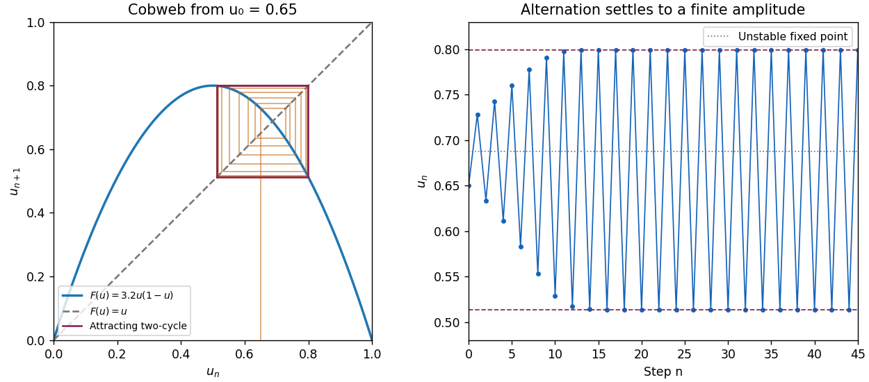
For $\lambda =3.2$, remove the fixed point factors from $F(F(u))-u$ to obtain ${\lambda }^2{u}^2-\lambda (\lambda +1)u+\lambda +1=0$. The resulting logistic map two-cycle isThese points map to each other. Their periodic-orbit multiplier is $F^{\prime }(u_{-})F^{\prime }(u_{+})=4+2\lambda -{\lambda }^2=0.16$, so the two-cycle attracts nearby iterates. The cobweb shows a small initial departure from $u_{\ast }=0.6875$ growing with alternating sign and then settling into the finite rectangle between $u_{-}$ and $u_{+}$. The time trace shows the corresponding finite-amplitude oscillation.