The Newton polynomial expresses the interpolation polynomial in products that successively vanish at all previously used interpolation nodes. With , the coefficients are divided differences:A triangular divided difference table computes all its coefficients using exactly divisions. The Newton polynomial and the Lagrange polynomial have the same polynomial degree bound and the same nodal values, hence are equal by uniqueness of polynomial interpolation.
For , , , the complete divided difference table isThe first divided differences are and , and their divided difference is . Reading the top entries givesThe initial term fits ; adding also fits ; adding fits while leaving the first two data values unchanged. This is the practical beauty of the Newton polynomial: each new correction respects all previous interpolation constraints.
If a new distinct interpolation node with value arrives, append one term:For example, appending to the three-point data gives , hence . Changing the order of the interpolation nodes changes the Newton polynomial coefficients and products, but not the final interpolation polynomial in exact arithmetic.
The products also permit nested evaluation analogous to Horner's method. If , start with and work backwards by ; the answer is . The three-point example becomes , needing two multiplications for each evaluation. This organization is useful when adding observations incrementally or evaluating a stored Newton polynomial many times; the Runge phenomenon still depends on the interpolation nodes rather than on which representation is used.
To justify the update formula, its added product vanishes at every previous interpolation node. Choosing by the new residual forces agreement at , so uniqueness of polynomial interpolation identifies the result. For , has polynomial degree at most , and the added product has leading coefficient one. Thus the new coefficient is exactly . The initial state is , with the empty product interpreted as one.[ref]
Appending to the four-point example in divided difference table leaves the Newton polynomial unchanged: , so the new fourth divided difference is zero. If the appended value is instead , the new coefficient isThis polynomial still takes values at the original interpolation nodes, and now takes value at . A zero update is a valid completed step: adding another exact sample of the original polynomial need not increase the polynomial degree.
Reordering the interpolation nodes changes the successive subsets used for the divided differences and the factors of the Newton polynomial. The final interpolation polynomial remains unchanged in exact arithmetic. For , reversing gives and values . The successive divided difference columns are nowFor example, the first second divided difference is . The top row becomes , givingThe earlier partial interpolants differ because they fit different subsets: fits , whereas fits . The highest divided difference is invariant because both complete top rows finish with the same set of four interpolation nodes; this is symmetry of divided differences.
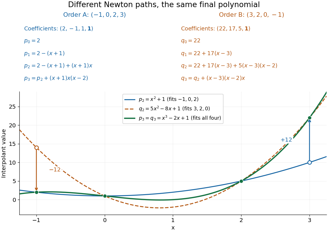
Reversing the interpolation nodes changes the Newton construction but gives the same final polynomial
. Details. This distinction is useful when checking a divided difference table: permuting all the interpolation nodes must preserve its final divided difference, even though the intermediate entries change. It also explains why data can be appended in their arrival order. In floating-point arithmetic, the subtractions and divisions may accumulate different rounding errors in different orders; exact invariance describes the mathematical polynomial, rather than guaranteeing bit-for-bit equality of numerical results.
Articles by others on the same topic


The Newton polynomial, also known as the Newton interpolation polynomial, is a form of polynomial interpolation that constructs a polynomial passing through a given set of points. It uses the concept of divided differences to express the polynomial and allows for the efficient computation of polynomial coefficients. The Newton polynomial is particularly useful for interpolating values at new data points, especially when new points are added dynamically, as it does not require recalculating the entire polynomial but can update it incrementally.