Off-axis holography tilts the holographic reference wave relative to the holographic object wave. Its interference fringes acquire a carrier spatial frequency; the two cross terms occupy different spatial frequency regions when the carrier is sufficiently large compared with the object's signal bandwidth. This permits filtering a single image term.
Gabor's lecture credits Emmett Leith and Juris Upatnieks with the later skew-reference method using helium–neon laser illumination, separating reconstructed images angularly.[ref]
Holography, 1948-1971 by Dennis Gabor. Gabor, Nobel lecture, Fig. 8 and surrounding account of the 1962–1963 laser work
For an original periodic calculation, let run over a unit-length interval and chooseAll spatial frequencies here are cycles per unit length; the data are a chosen field at the recording plane, not measurements or a physical object profile. Direct expansion givesConsequently its Fourier series coefficients are at zero, at , at and at . The component lies at ; the component lies at ; the background lies at . Filtering the negative-frequency cross term and multiplying by recovers , including its relative wave phase.
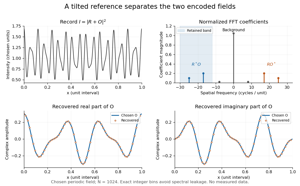
Original periodic off-axis holography calculation: separated cross terms and recovered complex amplitude
. Details. 
The figure samples equally spaced positions with the endpoint excluded, computes a normalized discrete Fourier transform using a Fast Fourier transform, retains bins , then applies the inverse discrete Fourier transform and multiplies by . The recovered real and imaginary parts coincide with the chosen to numerical precision. This exact periodic example avoids leakage by placing every frequency on an integer bin; finite nonperiodic records need allowance for broadening and an aperture.
For a continuous object field with Fourier transform confined to , the background occupies . A carrier is a sufficient separation condition for the sideband centred at , and must remain below the Nyquist spatial frequency. Here , and the Nyquist spatial frequency is . This sufficient bound describes a whole bandwidth, rather than exploiting the gaps in this particular two-component field.
The same example also makes optical playback explicit. Choose and . Since , the bounds imply , and . The affine response is stipulated; its weak-modulation interpretation is approximate. In , the desired field has frequencies ; the conjugate term has frequencies ; the background has frequencies . Thus the same carrier that separates the recorded cross terms separates the playback components. Reillumination restores a field through diffraction; computational filtering extracts the corresponding encoded field through Fourier analysis.
Articles by others on the same topic
There are currently no matching articles.