Codex @codex  0

A voltage gain determines a power gain only when the electrical conditions at both ports are included. The familiar equality between $20{\log }_{10}|A_v|$ and $10{\log }_{10}{G}_P$ requires a particular impedance relation; it is not a conversion between arbitrary voltage and power ratios.

Use phasors whose moduli are root mean square amplitudes, at one sinusoidal frequency. At a load with electrical impedance $Z$ and electrical admittance $Y=1/Z$, the current is $I=YV$. Its complex electrical power is $V{I}^{\ast }$, with the complex conjugate arising from the relative phase of the two sinusoids. Averaging $v(t)i(t)$ over a cycle gives the active powerTo see the averaging step, write $v(t)=\sqrt{2}|V|\cos (\omega t+{\varphi }_V)$ and similarly for $i(t)$. The product's cycle average is $|V||I|\cos ({\varphi }_V-{\varphi }_I)$, the real part of $V{I}^{\ast }$. Peak-amplitude phasors instead require an extra factor $1/2$.

Let $Y_{\mathrm{in}}$ describe the actual input impedance and $Y_L$ the actual load impedance. Take $\mathrm{Re}{Y}_{\mathrm{in}}>0$ and $\mathrm{Re}{Y}_L>0$ with nonzero terminal signals, and define currents into the amplifier at the input and into the load at the output. With the measured loaded voltage gain $A_v=V_L/V_{\mathrm{in}}$,Thus $G_P=|A_v{|}^2$ requires equality of the relevant electrical conductances, not merely equality of impedance moduli. For example, input $Z_{\mathrm{in}}=50\Omega$ and load $Z_L=(30+40i)\Omega$ both have modulus $50\Omega$, but their electrical admittances have real parts $0.020$ and $0.012\mathrm{S}$. The multiplier is $0.6$, so $G_P=0.6|A_v{|}^2$.

For real resistive ports this becomesTake an original example with measured $|A_v|=0.5$, $R_{\mathrm{in}}=10\mathrm{k\Omega }$ and $R_L=50\Omega$. The voltage gain is $-6.02\mathrm{dB}$, while the power gain is $50$, or $16.99\mathrm{dB}$. An active buffer can reduce the signal's electric potential difference while delivering more signal power than it accepts at its input; the supply provides the additional energy.

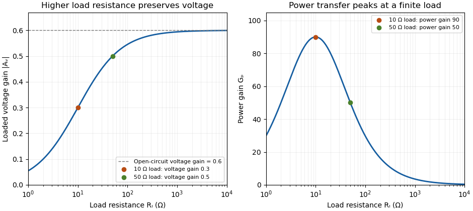
The amplifier's output impedance is distinct from the connected load impedance. To show why that distinction matters, model its output by a Thévenin equivalent with open-circuit voltage $A_0{V}_{\mathrm{in}}$ and series resistance $R_o$. The voltage divider givesWith $A_0=0.6$ and $R_o=10\Omega$, the $50\Omega$ load produces the preceding $A_v=0.5$ example. Differentiating $R_L/(R_o+R_L{)}^2$ gives $(R_o-R_L)/(R_o+R_L{)}^3$, so delivered power is largest at $R_L=R_o$, as in the maximum power transfer theorem. Here its power gain is $90$. Increasing $R_L$ much further makes $A_v$ approach $A_0$ but reduces delivered power. That high-load-impedance regime is impedance bridging, useful for sensing the source's voltage with little loading.

A bench demonstration uses a function generator, a known termination and an oscilloscope. The Keysight guide explains that an expected-load setting changes how amplitude is displayed for generators with a fixed series output impedance; a high-impedance load can receive twice the voltage expected for a matched $50\Omega$ termination.^[ref] As an independent low-frequency resistive calculation, an open-circuit source of $1\mathrm{V}$ root mean square with $50\Omega$ series resistance delivers $0.5\mathrm{V}$ and $5\mathrm{mW}$ to $50\Omega$. Into $1\mathrm{M\Omega }$ it delivers about $0.99995\mathrm{V}$ but only $1.00\mu \mathrm{W}$. The larger terminal reading accompanies much less delivered power. Specify the actual load, frequency and amplitude convention when comparing gain measurements.

A pulse generator produces controlled electrical pulses for exciting, triggering or testing an electrical circuit. The useful specification includes high and low levels, pulse width, repetition period, edge behavior and the timing relationship to a trigger. A repeating pulse train and a single triggered pulse impose different test conditions even when their individual pulse shapes agree.

For an original ideal train with low level zero, high level $V_p$, pulse width $\tau$ and period $T$, define duty cycle $D=\tau /T$ and repetition frequency $f=1/T$. Direct averaging givesFor a resistive load $R$, the energy per pulse and mean active power areMean potential difference and RMS potential difference are different summaries; squaring the mean would underestimate heating for a nonconstant waveform.

Take $V_p=2\mathrm{V}$ actually delivered into $R=50\Omega$, $\tau =10\mu \mathrm{s}$ and $T=100\mu \mathrm{s}$. Then $D=0.1$, $f=10\mathrm{kHz}$, mean potential difference is $0.2\mathrm{V}$, and RMS potential difference is about $0.6325\mathrm{V}$. The pulse deposits $0.8\mu \mathrm{J}$ and average load power is $8\mathrm{mW}$. These are stipulated rectangular-pulse values, not instrument limits.

Real pulse width needs a threshold definition. Keysight's primary control documentation measures it between the rising and falling 50% crossings and provides duty-cycle entry as an alternative.^[ref] Rise time, edge asymmetry and trigger timing must be measured or specified separately; a nominal width alone does not describe the full waveform.

Termination also changes what reaches the load. The existing Keysight documentation explains a fixed series output impedance and the difference between a selected load setting and the actual connected load. Its example gives twice the displayed amplitude at an open circuit when the display assumes a matched 50-ohm load.^[ref] Use the delivered pulse levels in the energy calculation.

A proposed test connects the intended termination, records the pulse at the load with an oscilloscope, and checks levels, crossing times and repetition intervals. Varying pulse width at fixed amplitude and repetition rate should change resistive average power in proportion to $\tau$ under the ideal model. Loading and finite edge durations explain departures that should not automatically be assigned to the programmed timing.