Loaded voltage gain is the ratio of an amplifier's output to input signal electric potential differences with a specified load connected. In a small-signal model, let the open-circuit output be and let the complete amplifier have output impedance . A load then givesThis is the voltage divider result from Thévenin's theorem at the output terminals. The university source explains why a linear circuit can be replaced at specified terminals by a source and series impedance.[ref]
Thevenin and Norton Equivalents, University of Houston teaching notes. pp. 1–2, The Idea and Important Notes
The output impedance used here must describe the complete amplifier at the stated operating point and frequency, including its feedback.The input terminal matters too. For a generator with source impedance driving amplifier input impedance , the corresponding source-to-load ratio in a unilateral model isThis includes both input and output loading; it differs from the terminal-to-terminal voltage gain defined above.
For an original resistive example, choose , , , and . The loaded terminal gain is , while the source-to-load gain is . Reducing the load to makes the terminal gain six, even though the stipulated open-circuit gain remains twelve. These are model parameters, not device specifications.
A direct test holds the actual amplifier input signal fixed, changes a known load and measures the output with an oscilloscope whose probe impedance is included in the effective load. Use small enough signals to retain linear operation and respect the amplifier output range. If the output-to-input ratio changes with loading, an unloaded gain alone is insufficient to predict the circuit's behavior.
At nonzero frequency the impedances and gain can be complex. A reactive-load phase shift in a finite-output-impedance amplifier can change both magnitude and phase, while input-output coupling or nonlinear current limiting can invalidate this simple unilateral divider model. The ideal feedback resistance-ratio examples in the manufacturer's introduction apply within their corresponding operating assumptions.[ref]
A reactive-load phase shift in a finite-output-impedance amplifier occurs because the load and output impedance form a frequency-dependent divider. In the model of loaded voltage gain, assume a positive real output resistance , an ideal capacitive load and open-circuit gain approximately constant over the band of interest. With ,The divider follows from the terminal equivalent described by the university circuit notes.[ref]
Thevenin and Norton Equivalents, University of Houston teaching notes. pp. 1–2, The Idea and Important Notes
Putting givesThus even an ideal capacitor can change both amplitude and phase when the source driving it has finite resistance. Its reactive current and energy exchange are described by complex electrical power; zero average dissipation in the ideal capacitor does not mean zero output-current demand.
For an original example, choose , and . Then and the load pole is . At that frequency the gain magnitude is and the extra phase lag is . A measured input of root mean square gives about root mean square at the capacitor, requiring approximately root-mean-square capacitive current.
A bench test holds the actual amplifier input fixed while sweeping frequency and compares loaded and unloaded output amplitudes and phases. Include probe capacitance in . The group delay introduced by a capacitive amplifier load also matters when comparing pulse waveforms.
This single-pole calculation assumes the stated constant open-circuit gain and resistive output impedance. The complete amplifier may have additional frequency dependence and feedback effects. The manufacturer's ideal feedback-gain examples are defined within their operating assumptions.[ref] Check the actual output-current and linear operating range before interpreting a departure from this model as a capacitor-only effect.
The group delay introduced by a capacitive amplifier load is the negative angular frequency derivative of the extra wave phase produced by that load. For the resistive output model in reactive-load phase shift in a finite-output-impedance amplifier, divide the loaded transfer function by the unloaded one:The added group delay is thereforeThis subtraction of unloaded wave phase prevents the amplifier's intrinsic group delay from being attributed to the capacitor. The terminal model uses a Thévenin equivalent; the group delay definition differentiates an unwrapped wave phase, as in the SciPy signal-processing documentation. Its digital-filter function reports samples, whereas the analog derivative above uses radians per second and gives seconds.[ref]
Thevenin and Norton Equivalents, University of Houston teaching notes. Printed pp. 1–2, terminal equivalence
[ref]SciPy 1.16.2 documentation. scipy.signal.group_delay, definition and Parameters: fs; discrete-frequency units
For an original example, choose and , hence . At , corresponding to , the added group delay is . The same operating point has : a single sinusoid's phase displacement and the delay of a narrow frequency packet need not agree.
A practical test applies a weakly modulated carrier, varies its central frequency, and measures the output modulation displacement while comparing loaded and unloaded operation. The group delay describes that narrow-band envelope only when the frequency response varies slowly across its bandwidth. The corresponding causal impulse response begins at zero time, for , and vanishes for ; it is not a rigidly translated impulse. Thus group delay versus pulse-front arrival for an RC load matters when a measured pulse is broad enough to change shape.
Group delay versus pulse-front arrival for an RC load distinguishes a narrow-band modulation displacement from the earliest response to a newly applied input. For the relative amplifier-load model in group delay introduced by a capacitive amplifier load, the causal impulse response is for and zero for . Its convolution with an input that vanishes before zero also vanishes before zero. Nevertheless its group delay is , which is positive and frequency dependent. The phase-derivative definition concerns spectral components and their envelopes.[ref]
An original finite-pulse calculation shows why a threshold measurement gives another time. For an initially relaxed load, apply a rectangular pulse of height and duration . Convolution givesThe first mathematical response occurs immediately after zero. A rising threshold equal to fraction of the input pulse height is reached at only if the pulse lasts at least that long. This is the threshold-crossing time of a finite rectangular pulse through an RC load.
With and , the largest output is only : a threshold is never reached. If instead, that threshold is crossed at . Neither value is the group delay evaluated at .
A pulse generator and oscilloscope can compare the threshold observation with a slow modulation on a carrier; the chosen threshold and modulation bandwidth must be recorded. MIT's laboratory likewise separates square-wave decay measurements from sinusoidal amplitude/phase measurements.[ref]
Laboratory 11: Sinusoidal Steady State Response of RC and RL Circuits by MIT OpenCourseWare. Printed pp. 1–2
If wiring adds a transport delay , shift the impulse response to : the front moves to , while the modulation delay becomes . The immediate onset of the unshifted lumped model is not a model of propagation along a finite-length cable.An electronic comparator registers a pulse only if its input reaches the chosen threshold. For an initially uncharged capacitor driven through an electrical resistance , a short rectangular pulse may end before that happens. The resulting threshold-crossing time of a finite rectangular pulse through an RC load depends on threshold and pulse duration, as well as the time constant ; it is not determined by group delay alone.
Take a positive input electric potential difference for , zero input outside that interval, and output across a capacitance . Include the source's effective series electrical resistance in . The initial condition is . Kirchhoff's voltage law and the capacitor current relation give the first-order linear differential equationThe output is a continuous function and reaches its maximum at the pulse's falling edge:The input jumps there, but an ideal capacitor's stored electric charge cannot change discontinuously under the finite currents of this model.
Choose a fixed threshold with . Solving the rising exponential function using a natural logarithm givesIf , the output never reaches the threshold. At , it touches the threshold only at its peak; the ideal time spent strictly above threshold is zero. A nonzero high interval in an ideal non-inverting electronic comparator requires . This is RC pulse-width discrimination: different input durations can give a missing pulse or a finite output pulse even when their input heights are equal.
For , solving the falling exponential decay givesHere is the time above threshold for an RC-filtered rectangular pulse, before any electronic comparator switching dynamics. It is not generally the input duration . Just above , differentiation gives and hence to first order; a half-height threshold gives slope two at the detection boundary.
For an original numerical example, take , , , and , so . A input peaks at only and is rejected. A input peaks at and givesThese are model calculations, not recorded instrument traces.
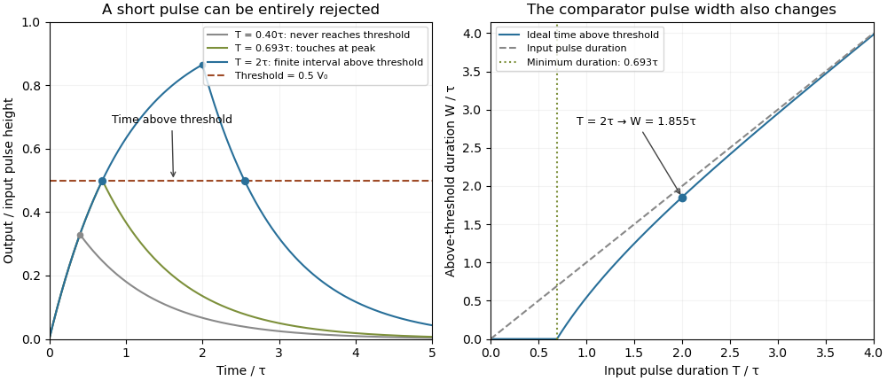

A threshold near the asymptotic input height is also especially sensitive to noise and threshold measurement uncertainty. Holding the absolute input height and fixed, the threshold timing sensitivity of an RC step response isFor the same , model, a effective threshold perturbation gives approximately of timing change at , but at , by first-order uncertainty propagation. The rectangular pulse must still last long enough to reach the selected threshold; changing together with is a different sensitivity calculation.
A bench test uses a pulse generator and an oscilloscope to record both the applied electric potential difference and the capacitor output. Sweep while keeping and the actual threshold fixed, and allow enough time between pulses for the measured initial output to be negligible at the desired precision. Include probe and comparator-input capacitance in . MIT's laboratory measures RC decay with a capacitor, a resistor and square-wave excitation; that gives a directly measurable component-value time constant.[ref]
Laboratory 11: Sinusoidal Steady State Response of RC and RL Circuits by MIT OpenCourseWare. Printed pp. 1–2, component values and decay/phase measurements
The pulse-duration sweep proposed here extends that decay measurement to a threshold observation. A real electronic comparator's input offset voltage, hysteresis and finite switching time must be separated from the ideal RC crossing times; a Schmitt trigger uses different rising and falling thresholds.RC pulse-width discrimination converts an input-duration test into a threshold observation on an RC circuit. For a relaxed first-order load with time constant , a positive rectangular input of height and duration reaches peak output . An ideal electronic comparator has a nonzero interval above fixed threshold precisely whenEquality only touches the threshold at the peak. The parent threshold-crossing time of a finite rectangular pulse through an RC load derives the full response and the rejected-pulse boundary.
This is a duration discriminator only while the input height is controlled. At a fixed duration, the same condition isA larger input can pass the threshold even when a smaller pulse of exactly the same duration fails. The minimum accepted duration decreases with height, with derivative .
For an original example, choose , , and . The minimum height for a nonzero comparator interval is about . A pulse peaks at about and is rejected; a pulse peaks at about and is accepted. Treating this observation as a width-only decision would conflate two different inputs.
A pulse-generator experiment therefore sweeps width at a recorded height and threshold, measures the actual capacitor waveform on an oscilloscope, and allows the initial state to relax. A residual baseline in RC pulse-width discrimination changes the next pulse's peak and invalidates the relaxed-state formula. Probe and comparator input capacitance also belong in the effective time constant. The natural-decay apparatus in MIT's RC laboratory supplies a direct component-level check of that time constant.[ref]
Laboratory 11: Sinusoidal Steady State Response of RC and RL Circuits by MIT OpenCourseWare. Printed pp. 1–2, square-wave decay and sinusoidal measurements
Comparator propagation delay and hysteresis are additional dynamics, not part of the ideal RC acceptance inequality.A capacitor need not finish discharging before the next pulse arrives. This residual baseline in RC pulse-width discrimination changes the next pulse's RC threshold-crossing time even if its applied height and duration are unchanged. The relaxed-state acceptance formula assumes an initial output of zero; a repeated pulse train can violate that assumption systematically.
Take a first-order RC circuit with time constant , input high level , zero input low level and initial capacitor output . During a pulse of duration ,For , solving for the rising threshold givesA finite interval above threshold requires . At equality the output only touches the threshold at its peak. A positive residual makes the crossing earlier than the zero-baseline crossing. If the output already exceeds the threshold at the start, this rising-crossing formula no longer describes a new edge.
The input of a repeated pulse train is a periodic function with high duration , low duration and period . Put and . The next baseline is the previous peak multiplied by . Writing for the baseline before pulse gives the linear recurrence relationBecause , the deviation from its fixed point is a decaying geometric sequence:This periodic RC pulse-train baseline is a repeatable state of the circuit, rather than random readout noise. In the periodic regime, separate rising and falling comparator transitions require . If , there is no finite high interval. If , there is no finite low interval: missing comparator reset in an RC pulse train can turn repeated input pulses into one sustained output state.
For an original calculation, choose , , , and . An isolated relaxed pulse peaks at only and is rejected. The repeatable train instead hasIts rising threshold occurs after each pulse starts. The falling crossing is , giving an above-threshold duration of . Starting from zero baseline, the first three pulses are rejected, but the fourth peaks at and crosses. A change in pulse acceptance need not mean that the source pulse itself changed.
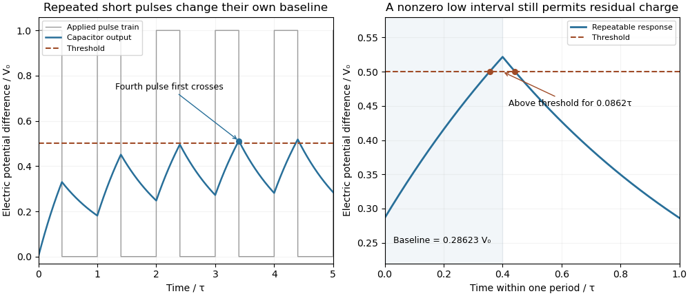
Residual capacitor charge makes a repeated short pulse cross a threshold that rejects the isolated pulse
. Original first-order model, with a 1 µs time constant, 0.4 µs high interval, 0.6 µs low interval and a half-height threshold. The first train starts relaxed; the second panel shows the repeatable baseline and peak. No measured waveforms are used. Details.
A useful design bound controls timing error rather than merely calling the circuit discharged. Put and suppose . Relative to the relaxed crossing,Since a nonnegative pulse train in this model has , a low interval guarantees that baseline bound. Combining the inequalities yields a sufficient quiet interval required for an RC baseline timing budget :For a 1% baseline allowance, limits the crossing advance to , or when . The bound is conservative because it uses the largest possible peak.
A bench test holds pulse height, duration and threshold fixed while sweeping repetition period with a pulse generator. Record the actual input and capacitor output on an oscilloscope, including the baseline immediately before each pulse. Probe capacitance and effective source electrical resistance belong in . MIT's laboratory uses repetitive square-wave excitation to measure RC decay, providing a direct way to check the underlying time constant.[ref]
Laboratory 11: Sinusoidal Steady State Response of RC and RL Circuits by MIT OpenCourseWare. Printed pp. 1–2, natural-response and waveform measurements
The calculations above assume ideal input edges and zero input low level; comparator hysteresis and switching dynamics require their own model.The quiet interval required for an RC baseline timing budget controls how much a residual capacitor baseline may advance the next threshold crossing. In residual baseline in RC pulse-width discrimination, a positive baseline changes the relaxed crossing byFor a permitted advance , requiring is equivalent to , where . To retain a fresh rising crossing, also require , equivalently .
After a previous peak , a zero-input low interval gives . Hence a measured upper bound on that peak gives the sufficient intervalUsing only the model bound recovers the conservative expression in the header, . The peak bound and initial-state assumptions are part of the guarantee. The next pulse must still last long enough to produce the rising crossing; this timing bound alone does not guarantee acceptance.
For an original timing budget, let , and . Then , and the conservative interval is . If a validated peak bound is only , it reduces to . Simply calling either interval several time constants long would hide the actual timing specification.
For , expansion gives under the full-height peak bound. Tightening a small timing allowance by a factor of two therefore adds roughly of quiet time. If the allowed advance is as large as the whole relaxed crossing time, a separate reset condition is still required; the logarithmic timing budget alone no longer ensures the initial output is below threshold.
A bench test measures the peak and the baseline while sweeping the low interval, keeping the threshold and pulse height fixed. MIT's RC laboratory supplies the natural-decay measurement used to check the underlying time constant.[ref]
Laboratory 11: Sinusoidal Steady State Response of RC and RL Circuits by MIT OpenCourseWare. Printed pp. 1–2, repetitive excitation and RC decay
Probe capacitance and source resistance belong in that measured time constant.Missing comparator reset in an RC pulse train occurs when the filtered output never spends a finite interval below the reset threshold between pulses. In the periodic first-order model, with and , the baseline is the minimum output and equalsFor a nonhysteretic ideal electronic comparator with , leaves no finite low interval. At equality the waveform merely touches the threshold. This is different from a pulse whose peak never reaches threshold and therefore gives no finite high interval.
Solving the strict reset condition givesSeparate rising and falling transitions also require the peak to exceed the threshold. Both inequalities matter, so increasing the quiet interval is not automatically sufficient to produce an accepted output pulse from a weak input.
For an original three-regime example, take , , and . The reset boundary is . At , the periodic baseline/peak are about : after startup the electronic comparator does not reset. At , they are , allowing both transitions. At , the peak is only about , so no finite high interval is produced. The same input height and high duration can therefore give three different output patterns as repetition changes.
The threshold-reset margin for a periodic RC pulse train must also accommodate uncertainty and switching dynamics. With a Schmitt trigger, the lower switching threshold controls reset while the upper one controls acceptance. The capacitor-level inequalities alone do not specify propagation delay or a real electronic comparator's minimum switching dwell time.
A test records the source, capacitor output and electronic comparator output together while sweeping . A steady high output with a pulsing input should be compared with the measured capacitor minimum before being attributed to a source failure. The RC decay model can be checked independently using the primary laboratory's natural-response method.[ref]
The threshold-reset margin for a periodic RC pulse train is the separation between the reset threshold of an electronic comparator and the largest baseline that the periodic RC low-pass filter may leave between pulses. A positive margin excludes missing comparator reset in an RC pulse train in the ideal threshold model; its size measures tolerance to additional electric potential difference errors.
Let be the input high level, the high duration, the quiet duration and the time constant. From the periodic solution in missing comparator reset in an RC pulse train, writeThis defines a margin in volts, rather than in units of standard deviation. If a nominal baseline has a known absolute error bound and the reset threshold has bound , a sufficient worst-case condition isThese are simultaneous bounds on the actual baseline and threshold. Adding their standard uncertainties would not by itself provide a deterministic guarantee; a probabilistic statement requires a specified joint probability distribution.[ref]
Guidelines for Evaluating and Expressing the Uncertainty of NIST Measurement Results by Barry N. Taylor and Chris E. Kuyatt. §§6.2–6.3, distributional conditions for interpreting uncertainty intervals
For an original example, let , and . Then , and the peak is . A threshold of gives . Bounds and leave . Raising the baseline bound to would remove this guarantee even though the nominal waveform still crosses the threshold.
A positive minimum separation does not specify the reset dwell time below threshold in an RC pulse train. A real electronic comparator needs enough time to switch, and the peak must separately exceed the acceptance threshold. For a Schmitt trigger, use the lower switching threshold in , while checking the upper one against the peak.
A focused bench test records the pulse generator output, capacitor output and electronic comparator output on an oscilloscope, then varies near the predicted boundary. Compare the measured minimum with the reset threshold and record the low interval as well as the minimum. The underlying exponential decay can be checked by the natural-response experiment in the MIT laboratory; the margin calculation above is an original application of that model.[ref]
Laboratory 11: Sinusoidal Steady State Response of RC and RL Circuits by MIT OpenCourseWare. Printed p. 1, capacitor response after switching and time-constant measurement
The reset dwell time below threshold in an RC pulse train is the continuous time for which the filtered electric potential difference lies below an electronic comparator's threshold between successive accepted pulses. A positive threshold-reset margin for a periodic RC pulse train ensures a crossing in the ideal model, but does not ensure a long enough low interval for the intended electronics.
Consider the periodic RC low-pass filter response to a high level lasting , followed by zero input for a quiet time . Let be the time constant, the periodic baseline at the start of the high interval and the peak at its end. Assume a nonhysteretic ideal electronic comparator and . Solving the two exponential segments gives the rising crossing time , measured from the high interval's start, and the falling crossing delay , measured from its end:The below-threshold interval runs from the falling crossing to the next rising crossing. ThereforeIncluding matters: the low interval usually extends into the next input high interval. The natural exponential decay underlying these segments is directly testable with the switched-RC apparatus in the MIT laboratory.[ref]
Laboratory 11: Sinusoidal Steady State Response of RC and RL Circuits by MIT OpenCourseWare. Printed p. 1, natural-response and time-constant experiment
For an original exact example, take , and . The periodic solution in missing comparator reset in an RC pulse train gives and . At , both crossing delays equal , so . The reset margin is a positive , yet a stipulated requirement of at least low time is not met.
The strict crossing assumptions are essential. At , the waveform only touches the threshold and the low interval vanishes. At or above the peak there is no finite high interval to separate. A Schmitt trigger uses distinct switching thresholds, so its output-state interval requires the corresponding falling and rising crossings rather than substituting one threshold indiscriminately.
A proposed measurement records the pulse generator, capacitor and electronic comparator outputs on an oscilloscope. Measure the low interval between actual output edges while also locating both capacitor-level crossings. Their difference can expose switching delays; the capacitor formula alone does not specify a real device's minimum pulse duration.
A periodic RC pulse-train baseline is the repeatable pre-pulse capacitor voltage reached after startup. It need not be zero even when the input low level is zero. With high duration , low duration , period , and , , the recurrence in residual baseline in RC pulse-width discrimination has contraction factor . Its fixed baseline and peak areThis is a deterministic periodic state, not a random noise floor. The startup error is reduced by a specified fraction after cycles, rounded upward.
The mean supplies an independent check. Integrating over a full period makes the derivative term vanish, so . The mean depends on duty cycle while the baseline and ripple depend on period relative to the time constant. For at fixed , expansion givesThus a rapid train approaches a level near its duty-cycle average, rather than isolated relaxed pulses.
For an original fast-train example, choose , , and . The exact baseline is about , the peak , and the mean exactly . The startup deviation contracts by each cycle; reducing it below one percent of its initial value takes 24 cycles, or .
A pulse-generator/oscilloscope test should therefore distinguish the first pulses from the repeatable train, and record minima, maxima and mean rather than only input width. The natural-response measurement in the primary RC laboratory checks the time constant used here.[ref]
Laboratory 11: Sinusoidal Steady State Response of RC and RL Circuits by MIT OpenCourseWare. Printed pp. 1–2
Threshold placement relative to the repeatable minimum and maximum determines acceptance and missing comparator reset in an RC pulse train.Threshold timing sensitivity of an RC step response measures how a crossing time changes when the absolute threshold or signal height changes. For a relaxed step response , with , the rising crossing isHolding the other inputs fixed givesA threshold approaching the step height encounters a flatter part of the exponential response, making the first sensitivity large.
For an original timing estimate, choose , , and effective small threshold-noise standard deviation . At , local linear propagation gives timing standard deviation about . At , it gives about . The latter threshold also needs a longer input pulse to be reached at all, as shown in threshold-crossing time of a finite rectangular pulse through an RC load.
The two voltage sensitivities can cancel under a different measurement calibration model. If the threshold is set to a fixed fraction of the same varying height, and , their contributions sum to zero. The crossing becomes , independent of amplitude in this ideal model. Such correlated threshold and amplitude errors in RC timing must retain covariance rather than add two independent voltage uncertainties.[ref]
The local noise rule also follows from dividing a small voltage perturbation by the crossing slope . It assumes a well-defined nearby crossing and sufficiently small perturbations; it does not describe multiple noise crossings, comparator switching dynamics, or a pulse ending before the threshold. A bench test can compare controlled threshold shifts with oscilloscope crossing times while holding the actual step height and initial state fixed.
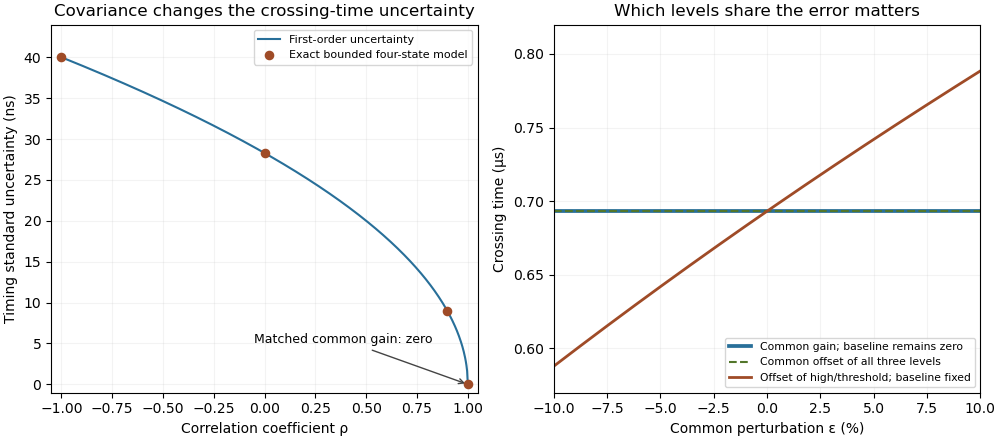
Covariance changes RC timing uncertainty, while gain and offset cancellation depend on the full measurement model
. Original calculation for a 1 V high level, 0.5 V threshold and 1 µs time constant. Exact four-state bounded-error checks are compared with first-order propagation. The right panel distinguishes common gain, a two-level offset with fixed baseline, and a common offset of all three levels. Its common perturbation sets gain or offset . No measured uncertainty data are used. Details.
A common offset in RC timing cancels only when every level used in the crossing model shares the same additive change. For high level , threshold , and initial baseline , assume and fixed time constant . The crossing time isAdding to all three levels leaves both differences unchanged, so the invariance in the header is exact. It describes a shared readout zero, or an equivalently translated step with a translated initial condition, rather than every possible physical offset experiment.
The three sensitivities make the cancellation visible locally:A common random offset has covariance matrix for these three inputs and contributes zero to the propagated timing variance. NIST's primary law retains exactly such covariance terms; setting them to zero would represent another measurement model.[ref]
For an original nonzero-baseline example, take , , and . The crossing is about . Adding to all three levels leaves it exactly unchanged. Adding the same offset only to and while keeping the baseline fixed instead increases it by about . The two-level sensitivity is , predicting to first order.
A calibration test must state whether the initial capacitor output, electronic comparator reference, input level and readout share the offset. Independent threshold errors, uncertainty of the time constant, and baseline memory remain even when this one common component cancels. The full distinction is developed in correlated threshold and amplitude errors in RC timing; a common gain is a separate invariance treated in ratiometric cancellation of RC timing gain errors.
Ratiometric cancellation of RC timing gain errors follows when the same positive gain multiplies every voltage level relevant to a threshold ratio. With zero initial baseline, fixed time constant , high level and threshold ,Replacing by with leaves and the time unchanged. This is an exact invariance, not merely the first-order cancellation of two uncertainty terms. It is a ratiometric measurement property of the specified model.
For an original example, choose , and . The crossing is approximately . Gains and both give the same result when they scale high level and threshold together. A shared readout gain can cancel from the calculated time in the same way; whether a reference also changes the physical circuit must be stated separately.
The mismatch remaining after common RC gain cancellation depends on the relative gains, not their common magnitude. Let the high level use gain and the threshold gain , with . Provided ,In the example, a one-percent relative mismatch delays the crossing by about , compared with from the first-order expression. Thresholds nearer the high level amplify the residual.
A nonzero initial baseline must share the gain too: is unchanged by multiplying all three levels by . Scaling only the high level and threshold against a fixed nonzero baseline is another experiment. Likewise, additive errors follow the conditions in common offset in RC timing, not the two-level scaling rule.
Uncertainty in the time constant, independent threshold error, baseline memory, and failure to reach the threshold remain even when one common gain cancels. Their covariance structure must follow the complete measurement model, as in correlated threshold and amplitude errors in RC timing and NIST's propagation law.[ref]
The mismatch remaining after common RC gain cancellation is the timing error caused by unequal gains in the amplitude and threshold paths after their common multiplicative part has canceled. It depends on their ratio, so improving a shared gain alone does not remove it.
For the zero-baseline RC threshold-crossing time, let with . If the amplitude is multiplied by and the threshold by , define the residual relative error by . The exact result from ratiometric cancellation of RC timing gain errors isHere is the time constant. As approaches one, the crossing is arbitrarily late; at or above one there is no finite rising crossing. An error budget must check this existence condition as well as a small timing residual.
For a new example, set , and . A one-percent positive mismatch gives ; a one-percent negative mismatch gives . The first-order estimate is , or here. The unequal exact magnitudes are a consequence of the logarithm, not an asymmetric tolerance specification.
If , monotonicity gives the exact worst absolute errorThus a bound in this example requires , about . This is a bound on the gain ratio, not on either gain separately.
For small fractional path errors , andA perfectly shared component has zero contribution to that difference. This is the law of propagation of uncertainty applied to the two gains; it does not cancel a change in , an additive threshold error or a nonzero unscaled baseline.[ref]
A proposed check varies the common gain while holding its ratio fixed, then varies only one path. Recording the two electric potential differences and the crossing on an oscilloscope distinguishes the exact common-gain invariance from the surviving mismatch.
The time above threshold for an RC-filtered rectangular pulse is the separation of its rising and falling threshold crossings, rather than the applied pulse duration. In the relaxed first-order model, put with and . The parent crossing calculation givesThis excludes comparator propagation dynamics and uses the same threshold on both edges. A Schmitt trigger with unequal switching thresholds needs a different formula.
The positive-width relation can be inverted exactly:Its derivative is . Thus a measured positive determines a unique input duration under the stated model. A zero-width observation does not: all rejected durations have that same outcome.
For an original example, take , and . The output remains above threshold for about , longer than the input pulse because of its decaying tail. Substitution into the inverse relation recovers .
For long pulses, tends to . It is positive below a half-height threshold and negative above one. At exactly half height, for every finite accepted pulse, with the difference tending to zero for long pulses. Consequently a measured above-threshold width cannot be equated to the input width without the threshold and filter model.
A pulse-generator/oscilloscope comparison can record both widths while varying threshold. The measured RC decay should be checked independently, using the natural-response method in the primary MIT laboratory.[ref]
Laboratory 11: Sinusoidal Steady State Response of RC and RL Circuits by MIT OpenCourseWare. Printed pp. 1–2
Initial residual charge, hysteresis, and different rising/falling comparator delays alter the observation; the algebra above only inverts the ideal capacitor waveform. Articles by others on the same topic
There are currently no matching articles.