Solutions to the paper whose cover dates the examination to 6 June 2015, 2:30–4:00 pm. Source: released examination archive, member
2015-cafv.pdf. All three questions are covered, although candidates were asked to attempt at most two. In the binary decision diagrams, dashed arrows mean zero and solid arrows mean one. In the linear temporal logic calculations, , and .Follow the binary decision diagram from its top decision node to a terminal node, choosing the outgoing arrow specified by each tested Boolean variable. If , the left decision node returns , independently of . If , the right decision node returns one when and otherwise returns . Thus the truth table, with rows in the order , is:
Thus the output column of the truth table, in the displayed order, is . In particular, the skipped test on the left does not constrain : both values give the same result.
Splitting the Boolean function according to the first tested Boolean variable givesThe identity follows by considering and . Using it and distributing Boolean conjunction over Boolean disjunction,The first two terms combine to because . This also explains the truth table: always makes the output one, while with the output is one exactly when both and are one.
For a complete binary decision tree with variable ordering of a binary decision diagram , first test , then , then on every branch. The four Boolean cofactors after the first two tests are
The eight terminal nodes, read from left to right in the figure, are . The repeated tests are intentional: this is the full binary decision tree before any reduction.
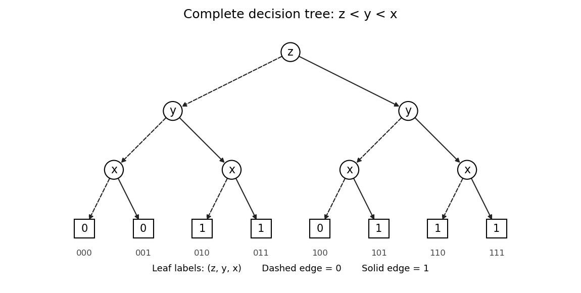

For example, the branch ends at one, whereas ends at zero. This checks the dependence on that must survive the later reduction.
A reduced ordered binary decision diagram is obtained by sharing equal terminal nodes, removing a decision node whose two children are equal, and sharing decision nodes with the same tested Boolean variable and the same ordered pair of children. Apply these rules to the binary decision tree in part (c) as follows.
- Merge the three zero terminal nodes into one zero terminal node, and merge the five one terminal nodes into one one terminal node.
- At the decision node has children . Remove it and redirect its incoming arrow to zero.
- At and the two decision nodes each have children . Remove both and redirect their incoming arrows to one.
- The remaining decision node, at , has children , so retain it.
- The decision node under now has children , while the one under has children . These are different, so neither can be merged or removed. The top decision node also has different children.
The left panel below is therefore the resulting reduced ordered binary decision diagram. Its full description is
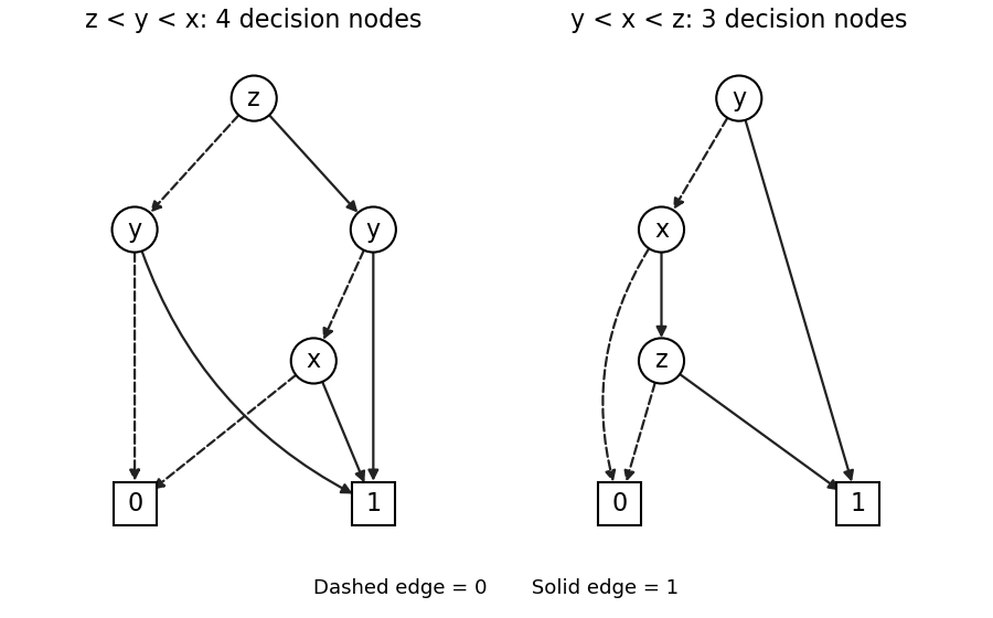
Reduced ordered decision diagrams: reversing the given order preserves its size, while testing y first saves one decision node
. Details. 
The original binary decision diagram also has four decision nodes and two terminal nodes, and is already reduced for : the two decision nodes have different children and no decision node has two equal children. Thus reversing the order has not made this example smaller. Indeed is unchanged by interchanging and , and the new binary decision diagram is the original one with those two labels exchanged. The uniqueness of a reduced ordered binary decision diagram applies to a fixed variable ordering of a binary decision diagram; it does not assert that every ordering has the same size.
Choose the variable ordering of a binary decision diagram . The Boolean cofactor with is the constant one, while the Boolean cofactor with is . Consequently the right panel in part (d) has the following arrows:Here an entry such as denotes the zero arrow to the decision node. There are vertices: three decision nodes and two terminal nodes, saving one decision node relative to either of the previous orderings. Testing first is effective because its one branch settles the entire Boolean function immediately. The ordering works equally well.
This is also minimal among ordinary binary decision diagrams for this Boolean function. Each Boolean variable is essential: setting leaves ; setting leaves ; and setting leaves . If a Boolean variable were never tested, the represented Boolean function could not depend on it. Thus at least three decision nodes are necessary, and the construction attains that bound.
A transition relation requires an explicit interpretation of the Boolean variables as current and next state bits. Take the four states . Encode the current state by and the next state by , and defineThe extra current bit is deliberately unused by the Boolean formula. A four-state transition system normally needs four bits to describe a pair of states; a Boolean formula using only three of them simply describes a transition relation independent of the fourth bit.
When , the condition is , so the permitted next states are and . When , the condition is , so the permitted next states are . The resulting adjacency matrix, with rows and columns both ordered , isThe directed graph below plots all ten directed edges, including the three self-loops. No arrow enters , but it is a valid state with two outgoing arrows. Every state has a successor. As permitted, no initial states are distinguished.
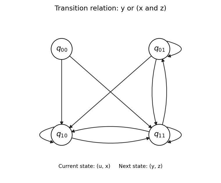
Four-state transition system with current bits (u, x), next bits (y, z), and relation y or (x and z)
. Details. 
Use the two incoming initial arrows in the source figure: . An atomic proposition is true precisely at the states whose displayed labels contain it. In particular, is false at every state. Hence is true on every infinite path in a transition system, and the first implication in the fairness assumption imposes no restriction.
Write . The remaining implication is . By the linear temporal logic duality , it is equivalent tosince implies . Thus a path is fair exactly when it visits states not labelled with both and infinitely often. This condition also follows directly: if eventually holds forever, then eventually holds forever and the required is impossible; if does not eventually hold forever, the implication has a false antecedent.
Every initial path in a transition system in the upper component either alternates forever between and , or makes finitely many alternations and then stays at . These are all fair: the first visits infinitely often, and the second visits infinitely often; neither state satisfies .
In the lower component, a path in a transition system can stay at forever, or leave it after finitely many visits and pass through to . The constant path in a transition system is unfair because holds forever while never holds. Every departing path in a transition system is fair because satisfies neither nor . Here means infinite repetition of the finite word . ThereforeThis notation lists initial paths in a transition system. If one instead allows arbitrary starting states, their suffixes starting at are fair as well; the fair paths in a transition system from each initial state, and hence all verdicts below, are unchanged.
Denote the three families found in part (a) by , and , where . All are fair paths in a transition system. The verdicts areEach verdict follows from the infinite path in a transition system semantics, rather than from a finite prefix alone.
For , take . From onwards, is always false, so there is no time after which is always true. Therefore the first specification fails, with fair counterexample . The path in a transition system is another fair counterexample, because it encounters , where is false, infinitely often. Each does satisfy , since satisfies forever.
For , take . Its next state is , so is true, but is false as just shown. Thus the second specification fails, with fair counterexample . Alternatively, has next state , making its antecedent true and its consequent false. For with , the next state is still , so this implication is true there because its antecedent is false; this does not rescue a universally quantified specification.
For , the fair path in a transition system reaches , where is false. Thus the third specification fails, with fair counterexample . In fact every fair initial path in a transition system reaches or , so none satisfies .
For , strong until requires an eventual position satisfying , together with at every earlier position. On , is true forever, so never holds. Thus the fourth specification fails, with fair counterexample . On each , holds until entry into , after which holds forever. On each , holds until entry into , after which holds forever. These latter paths in a transition system satisfy the strong until requirement.
For , weak until permits either the preceding strong until behavior or . Every and satisfies the strong until behavior, and satisfies . These exhaust the fair initial paths in a transition system. Therefore the fifth specification holds on every fair initial path. Allowing the left operand to continue forever is exactly what distinguishes this answer from the previous one.
For , the two next-time operators belong to the left operand of strong until. The fair path in a transition system has true at positions zero and one, then false at every position from two onwards. Therefore first holds at position two. But is false already at position zero, since is false at position two. A witness for strong until cannot occur at zero or one, where its right operand is false, or at two or later, where its left operand has already failed. Thus the sixth specification fails, with fair counterexample .
Indeed, every fair initial path in a transition system fails the sixth specification. On , the right operand never holds. On and , let be the first position of the permanent tail. The left operand is false at , strictly before any possible right-operand witness. This also checks that the two next-time operators cannot be ignored or shifted onto the whole strong until formula.
To apply bounded model checking, seek an initial path in a transition system satisfyingA satisfying assignment for its bounded encoding is enough to disprove the specification. Use a lasso path: positions follow the transition relation, and a final arrow returns from to some , . The repeated part is . On such a lasso path, is equivalent to having true at some position of the repeated part.
For this example an explicit Boolean formula for the bounded search isHere means and means that the source diagram has the arrow ; each can be encoded by finite Boolean variables for the states. The loop requirements are the fairness assumption and the negated specification respectively. Unrolling the transition relation and adding a loop closure is the usual bounded model checking construction.[ref]
Symbolic Model Checking without BDDs by Armin Biere and others. §2, worked example with an unrolled transition relation and a returning loop; §3, infinite-path semantics
At bound , an initial self-loop would be needed. The only such choice is , whose repeated label satisfies and . It violates both loop requirements. The other initial state, , has no self-loop. Thus has no satisfying assignment.
At bound , chooseBoth required arrows and exist. At , is false and hence is false, so both repeated-part requirements are true. Equivalently, the label values are and . These values give a satisfying assignment of , representing the fair counterexample . ConsequentlyHere the bound counts forward arrows before the returning arrow, so stores two positions and describes a two-state repeated part. There is no need for a completeness bound: the exhibited fair counterexample settles the negative answer. These satisfying assignments are checked directly; no claim of executing an external SAT solver is needed.
Write . All arguments depend only on this given satisfaction set; they do not require an additional convention for the printed notation . For a state , let . The power set is ordered by set inclusion.
Take and any . By the definition of , we have both and . By transitivity of set inclusion, , so . Since this applies to every member of ,Thus is an order-preserving function, which is the meaning of monotonicity here. This proof does not need either finiteness or the absence of terminal states.
Let . By computation tree logic semantics, a state belongs to exactly when every infinite path in a transition system starting there stays in at every position, including position zero. There are no terminal states, so every state lies at the start of an infinite path in a transition system.
If , then . For any successor of , every infinite path in a transition system from can be prefixed with . Hence every such continuation stays in , so . Thus and .
Conversely, if , then and every successor belongs to . Every infinite path in a transition system from therefore has its first state in and its entire remaining tail in . Consequently . Both inclusions giveso the desired satisfaction set is a fixed point of .
Every state has at least one successor, so for every . ThereforeThe empty set is always a fixed point. Whenever is nonempty, it is therefore an additional, distinct fixed point.
For an explicit example, take a one-state transition system with , the self-loop , and . Then and has the two distinct fixed points and . This example meets the requirement of no terminal states.
The wording does not guarantee distinct additional fixed points for every instance. For example, if , then for every and its only fixed point is . Thus additional fixed points can occur, but need not occur. The universal example is distinct precisely when the desired satisfaction set is nonempty, as also follows from the greatest fixed point argument below.
Let be any fixed point of . Thenso and every successor of every member of belongs to . Take and an arbitrary infinite path in a transition system from . By mathematical induction, every belongs to : the base case is the choice of , and implies .
Since , the whole path in a transition system stays in . The path in a transition system was arbitrary, so . Thus , and since was arbitrary in ,Part (b) proves that itself is a fixed point. Thereforethe greatest fixed point with respect to set inclusion. In fact the same induction works for every , showing why a successor-closed set of good states certifies this universal property.
Start with every state, and repeatedly discard a state that is outside or has any successor outside the current candidate set. Use a fresh set on each iteration so that the displayed procedure computes exactly :This is fixed-point iteration , . The first step gives , because every successor is a state of . Thus . If , the order-preserving function property givesThe candidate sets therefore form a descending chain under set inclusion.
function Sat_AG(S, Post, A):
    X = copy(S)
    repeat:
        Y = empty_set()
        for s in S:
            if s in A and every t in Post(s) belongs to X:
                insert s into Y
        if Y == X:
            return X
X = YEvery fixed point is contained in every : initially , and implies . At return, , and contains every fixed point. The returned set is consequently the greatest fixed point, so by part (d).
The iteration also has a direct interpretation. contains precisely the states satisfying now; retains those satisfying it now and at all immediate successors; later rounds extend the checked horizon one step at a time. The stable set enforces the condition at every future position.
Yes: the procedure always terminates after finitely many steps. If an iteration does not return, then . Thus at least one state is permanently removed. A finite set of states can suffer at most such strict decreases, after which the next equality test must return. Therefore the procedure makes at mostwhen started from , counting the final evaluation that detects equality. The bound also covers , where the first evaluation already returns. Each evaluation inspects finitely many states and successors, so every individual step terminates as well. Finiteness, rather than monotonicity alone, supplies this finite termination bound.
Articles by others on the same topic
There are currently no matching articles.