Past exam of the computer science course of the University of Oxford / 2015

a

Solution

The accounting method assigns each operation a charge, its amortized cost, that can differ from its actual cost. Cheap operations save the excess charge as credits associated with the data structure or its entries. An expensive operation spends these previously saved credits. The essential invariant is that the credit balance never becomes negative.

If the initial balance is zero, operation

i

has actual cost

c_{i}

, charge

c_{i}

, and leaves balance

B_{i}

, then

B_{i} = B_{i - 1} + c_{i} - c_{i}, \sum_{i = 1}^{n} c_{i} = \sum_{i = 1}^{n} c_{i} - B_{n} \leq \sum_{i = 1}^{n} c_{i} .

Thus a nonnegative credit balance makes the total charge an upper bound on the total actual cost for every operation sequence. In particular, a constant time charge proves a linear time total. The argument is a deterministic amortized analysis; it requires no probability distribution on the operations. A nonzero initial balance must be included as an additive term in the bound.

b

Solution

Yes: starting from zero, $n$ increments of the decimal counter cost $Θ (n)$ digit changes, uniformly in the number

k

of digits. An increment changes the trailing digits equal to

9

into

0

and increases the next digit. Number digits from

0

at the least significant end. Digit

i

changes once every

1 0^{i}

increments, so the exact number of changes is

C_{10} (n, k) = \sum_{i = 0}^{k - 1} ⌊ \frac{n}{1 0 ^{i}} ⌋ \leq n \sum_{i = 0}^{\infty} 1 0^{- i} = \frac{10 n}{9} .

Here the floor function counts carries reaching each position, and the last equality sums a geometric series. Since digit

0

changes on every increment,

C_{10} (n, k) \geq n

for

k \geq 1

. The loop tests and carry handling add only a constant amount per changed digit and per operation, giving the same time complexity.

An accounting method explanation is also possible. Charge two credits for each change of digit

0

: one pays for that change and one joins a common bank. For

n

increments the higher digits change at most

n /9

times, so their costs can be covered from that bank; the displayed prefix bound ensures that it never goes negative.

The formula allows wraparound modulo

1 0^{k}

; alternatively, restrict to increments before overflow. Initializing the array itself costs

Θ (k)

if that is counted separately. If the initial digits are arbitrary, the number of changes at position

i

is at most

⌈ n /1 0^{i} ⌉

, giving

O (n + k)

in Big O notation. Starting with all digits equal to

9

makes the first increment cost

k

, so the initial-state convention matters.

c

Solution

For an initially zero binary counter, bit

i

changes precisely on increments whose indices are divisible by

2^{i}

. Weighting each such change by

2^{i}

gives the exact total

C (n, k) = i = 0 \sum k - 1 2^{i} ⌊ \frac{n}{2 ^{i}} ⌋ .

For

n \geq 1

and

k \geq 1

, put

r = min {k, 1 + ⌊ lo g_{2} n ⌋}

. All summands with

i \geq r

vanish; each of the other summands is at most

n

. Therefore

C (n, k) \leq n r = O (n min {k, 1 + lo g_{2} n}) .

This is sharper than simply charging

n

for each of all

k

positions when

n

is small. To show that the order is best possible, use

⌊ x ⌋ \geq x /2

for

x \geq 1

. For every

0 \leq i < r

2^{i} ⌊ \frac{n}{2 ^{i}} ⌋ \geq \frac{n}{2}, \frac{n r}{2} \leq C (n, k) \leq n r .

Thus the asymptotic analysis gives a tight bound. If wraparound is excluded,

n < 2^{k}

, and this becomes

Θ (n (1 + lo g_{2} n))

, often written

Θ (n lo g n)

for

n \geq 2

. If wraparound is allowed and

n \geq 2^{k}

, it becomes

Θ (nk)

. For

n = 0

, the cost is zero.

For completeness, the same conclusion cannot be asserted uniformly over arbitrary initial binary counter states. An initial value

2^{k} - 1

makes the first increment change every bit, costing

2^{k} - 1

. A general upper bound follows by replacing each floor function in the count by a ceiling function:

C_{arbitrary} (n, k) \leq \sum_{i = 0}^{k - 1} 2^{i} ⌈ \frac{n}{2 ^{i}} ⌉ \leq n r + 2^{k} - 1.

To see the second inequality, split at

r

: for

i < r

, use

⌈ n / 2^{i} ⌉ \leq n / 2^{i} + 1

, and for

i \geq r

, use

⌈ n / 2^{i} ⌉ = 1

. For

n \geq 1

the worst initial-state cost is consequently

Θ (n r + 2^{k})

. This qualification separates initialization from the usual amortized analysis starting at zero.

d

Solution

Use two permanent stacks,

F

and

B

, and one temporary stack,

T

. At operation boundaries

T

is empty. Maintain the representation invariant that the deque, read from front to back, is the top-to-bottom contents of

F

followed by the bottom-to-top contents of

B

. Thus the tops of

F

and

B

are the two accessible ends. Maintain their sizes using two counters, requiring only

O (1)

additional storage in Big O notation.

Adding at the front pushes onto

F

; adding at the back pushes onto

B

. Removing at an end whose permanent stack is nonempty simply pops that stack. If both permanent stacks are empty, report an empty deque.

Suppose a front removal finds

F

empty and

B

contains

m > 0

elements. Rebalance as follows:

Move the top $⌊ m /2 ⌋$ elements of $B$ onto $T$ .
Move all remaining $⌈ m /2 ⌉$ elements of $B$ onto $F$ .
Move all elements of $T$ back onto $B$ .
Pop and return the top of $F$ .

The parked elements are the back half of the deque; the unparked elements are the front half. Moving the front half onto

F

reverses their stack order and exposes the correct front element. Parking and restoring the back half reverses it twice, preserving its original order in

B

. The temporary stack is empty again. For a back removal with

B

empty, exchange the roles of

F

and

B

throughout. Rebalance approximately half the elements, so both ends retain accessible elements after a large transfer.

For the amortized analysis, count each push or pop as one unit and use the potential method with

Φ = 3 ∣ F ∣ - ∣ B ∣ .

Initially the deque is empty, so

Φ = 0

, and

Φ

is always nonnegative. An ordinary insertion or removal costs one unit and changes the size difference by at most one, giving amortized cost at most

4

For a rebalancing removal, let

h = ⌊ m /2 ⌋

. The parked half makes two transfers per element and the other half makes one; each transfer is a pop and a push. Including the final removal, the actual cost is

c = 4 h + 2 (m - h) + 1 = 2 m + 2 h + 1 \leq 3 m + 1.

Before rebalancing the absolute size difference is

m

. Immediately after the split it is at most

1

, and after the removal it is at most

2

. Hence

c = c + ΔΦ \leq (3 m + 1) + 3 (2 - m) = 7.

Size tests and counter updates change only these constants. Summing the amortized costs and using nonnegative final potential proves $O (1)$ amortized running time for all four operations, with three stacks and $O (1)$ additional storage. An individual rebalancing operation can still take linear time in the current size.

2

a

Solution

A flow network is a finite directed graph

G = (V, E)

with nonnegative flow network edge capacities

c_{e}

, together with distinct source and sink vertices

s, t

. A feasible flow in the nonnegative directed-edge convention is a function

f : E \to R_{\geq 0}

satisfying the capacity constraints and flow conservation:

0 \leq f_{uv} \leq c_{uv} (uv \in E), \sum_{u : uv \in E} f_{uv} = \sum_{w : v w \in E} f_{v w} (v \in / {s, t}) .

Its flow value is the net outflow at the source,

∣ f ∣ = \sum_{w : s w \in E} f_{s w} - \sum_{u : u s \in E} f_{u s},

which equals the net inflow at the sink by flow conservation.

A cut of a flow network is a partition of a set

(S, V ∖ S)

with

s \in S

and

t \in / S

. Its cut capacity counts only directed edges leaving

S

c (S, V ∖ S) = \sum_{u \in S, v \in / S : uv \in E} c_{uv} .

The net flow across the cut of a flow network subtracts flow on edges returning into

S

, and equals

∣ f ∣

For the following parts, a circulation with vertex demands has no exceptional source or sink in the original directed graph. Instead it satisfies net inflow minus net outflow equal to

d_{v}

at every vertex. Thus positive demands consume flow, and negative demands supply flow.

b

Solution

Write flow balance using the positive-inflow convention

\sum_{u : uv \in E} f_{uv} - \sum_{w : v w \in E} f_{v w} = d_{v} .

Remove the lower bounds on network flow by writing

f_{uv} = ℓ_{uv} + x_{uv}

, where only

ℓ_{BC} = 4

is nonzero. Then

0 \leq x_{uv} \leq c_{uv} - ℓ_{uv}

, and its required flow balance is

d_{v}^{'} = d_{v} - (\sum_{u} ℓ_{uv} - \sum_{w} ℓ_{v w}) .

In the order

A, B, C, D

, the lower-bound contribution is

(0, - 4, 4, 0)

, so

(d_{A}^{'}, d_{B}^{'}, d_{C}^{'}, d_{D}^{'}) = (- 6, 1, 0, 5) .

The resulting flow network edge capacities are

c_{A B}^{'} = 5, c_{A C}^{'} = 2, c_{BC}^{'} = 5, c_{B D}^{'} = 3, c_{C D}^{'} = 5.

Add a new source

s

with an edge

s \to A

of flow network edge capacity

6

, and a new sink

t

with edges

B \to t

and

D \to t

of flow network edge capacities

1

and

5

. A feasible flow saturating these new edges is equivalent to a solution for

x

: ordinary flow conservation in the enlarged flow network produces exactly the residual supplies and demands above. All source and sink edges must be saturated, requiring flow value

6

Figure 1.
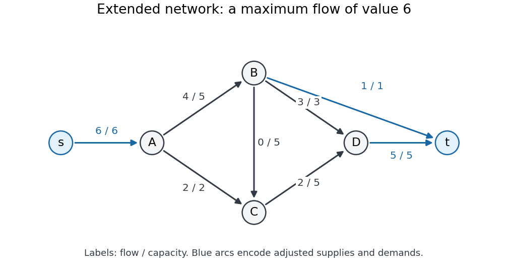
Extended flow network after removing the lower bound; labels show final flow divided by flow network edge capacity
. The auxiliary edges are blue. The displayed flow saturates the auxiliary source and sink edges, certifying that all adjusted demands are met. The original edge $BC$ regains its four-unit lower bound only after this auxiliary problem is solved. **Details**.

Start the Edmonds–Karp algorithm at zero flow. Repeated breadth-first search in the residual network permits the following shortest augmenting paths; when paths tie, choose the one through

B

first.

Step	Augmenting path	Added flow	Total flow value
$1$	$s \to A \to B \to t$	$min (6, 5, 1) = 1$	$1$
$2$	$s \to A \to B \to D \to t$	$min (5, 4, 3, 5) = 3$	$4$
$3$	$s \to A \to C \to D \to t$	$min (2, 2, 5, 2) = 2$	$6$

The first augmenting path has three edges. Once

B \to t

is saturated, the next shortest possibilities have four edges, so steps

2

and

3

respect the breadth-first search rule. Each augmentation adds the usual backward edges to the residual network, though these particular augmentations need only forward edges. Now

s \to A

is saturated, so no further augmenting path exists. The cut of a flow network with source side

{s}

has cut capacity

6

, proving that the obtained flow is a maximum flow.

The original-edge values for

x

are

(4, 2, 0, 3, 2)

in the order

A B, A C, BC, B D, C D

. Restore the lower bound to obtain

(f_{A B}, f_{A C}, f_{BC}, f_{B D}, f_{C D}) = (4, 2, 4, 3, 2) .

All original capacity constraints hold, and

f_{BC} = 4

meets its lower bound. The net inflows at

A, B, C, D

are respectively

- 4 - 2 = - 6, 4 - 4 - 3 = - 3, 2 + 4 - 2 = 4, 3 + 2 = 5.

(6)

The original network therefore admits a feasible circulation with vertex demands.

c

Solution

For any feasible circulation with vertex demands, sum its defining flow balance over all vertices:

\sum_{v \in V} d_{v} = \sum_{v \in V} \sum_{u : uv \in E} f_{uv} - \sum_{v \in V} \sum_{w : v w \in E} f_{v w} .

Every directed edge

ab \in E

contributes

+ f_{ab}

exactly once to the first sum, at its head

b

, and

- f_{ab}

exactly once to the second, at its tail

a

. The two sums therefore contain exactly the same terms. They cancel, giving

v \in V \sum d_{v} = 0.

This is global flow conservation: internal transport cannot create or destroy the total amount. Lower bounds on network flow and capacity constraints restrict which flows are feasible but do not affect the cancellation. The condition is necessary, not sufficient: insufficient flow network edge capacities can still prevent satisfying balanced demands.

d

Solution

For each user define its set of eligible ads by

E_{i} = {j : S^{i} \cap S_{j} \neq = \emptyset} .

This uses the intersection of demographic-group memberships: belonging to one advertised group suffices, because the eligibility condition is a set union. A user in several groups still receives at most one ad.

A direct algorithm is to process users independently. For user

u_{i}

, scan ads

a_{j}

until finding one for which some group

S_{ℓ}

belongs to both

S^{i}

and

S_{j}

. Assign that ad and stop processing this user. If no such ad exists, leave the user unassigned. There is no upper bound on the number of different users who can receive the same ad, so these decisions do not compete for an ad resource.

For correctness, every produced impression has a shared permitted group, and the stopping rule assigns at most one ad to each user. Conversely, a user with

E_{i} = \emptyset

cannot receive an ad in any feasible solution. Since every other user can contribute at most one impression, every feasible solution has value at most

{i : E_{i} \neq = \emptyset} .

The algorithm attains this bound, proving

maximum impressions = {i : S^{i} \cap S_{j} \neq = \emptyset for some j} .

Represent each membership set by a length-

k

array of Boolean variables. Testing one user-ad pair costs

O (k)

, so all tests and input setup take

O (nmk + (n + m) k + n + m + k)

time in Big O notation, which is polynomial time in all three parameters. For positive

n, m, k

, this simplifies to

O (nmk)

A maximum flow formulation gives the same result if desired: add edges

s \to u_{i}

with flow network edge capacity

1

u_{i} \to a_{j}

with flow network edge capacity

1

exactly when

j \in E_{i}

, and

a_{j} \to t

with flow network edge capacity

n

. By the integral max-flow theorem, an integral maximum flow selects valid impressions. Setting the last flow network edge capacity to

1

would impose an extra restriction absent from this paper.

3

a

Solution

Using the standard maximum form of a linear program, write

max c^{T} x subject to A x \leq b, x \geq 0,

where

x \in R^{n}

A \in R^{m \times n}

b \in R^{m}

, and

c \in R^{n}

. The inequalities are coordinatewise, and

c^{T} x

is the objective function. General linear programs can be put in this form: reverse the sign of a minimization objective function, reverse lower-bound linear inequalities, replace an equality by two opposite linear inequalities, and replace each unrestricted variable by the difference of two nonnegative variables. Some conventions instead call the equality-constraint version standard form; the convention here is the maximum-with-upper-bounds convention.

Introduce nonnegative slack variables

x_{n + i} = b_{i} - \sum_{j = 1}^{n} a_{ij} x_{j}

. The equivalent slack form of a linear program is

z x_{n + i} x_{j} = j = 1 \sum n c_{j} x_{j}, = b_{i} - j = 1 \sum n a_{ij} x_{j} (1 \leq i \leq m), \geq 0 (1 \leq j \leq n + m) .

The original variables are initially nonbasic and the slack variables basic. More generally, a slack form of a linear program specifies disjoint index sets

N, B

and writes

z = v + \sum_{j \in N} c_{j} x_{j}, x_{i} = b_{i} - \sum_{j \in N} a_{ij} x_{j} (i \in B), x_{i} \geq 0 (i \in N \cup B) .

Thus each basic variable and the objective function are expressed using only nonbasic variables. Setting all nonbasic variables to zero gives the associated basic solution, which is a feasible solution exactly when the resulting basic values are nonnegative. The slack form of a linear program does not itself require that initial basic solution to be feasible.

b

Solution

A vertex cover of an undirected graph

G = (V, E)

is a subset

C \subseteq V

containing at least one endpoint of every edge. The optimization version of the vertex cover problem minimizes

∣ C ∣

; the vertex cover decision problem asks whether a cover of size at most a given bound exists.

Let

x_{v} = 1

mean that vertex

v

is selected. An integer program for minimum-size vertex cover is

min subject to v \in V \sum x_{v} x_{u} + x_{v} \geq 1 x_{v} \in {0, 1} (uv \in E), (v \in V) .

The linear programming relaxation replaces

x_{v} \in {0, 1}

0 \leq x_{v} \leq 1

. The edge inequalities enforce coverage, and the objective function counts selected vertices in the integer program.

For a graph triangle with vertices

1, 2, 3

, the three covering constraints are

x_{1} + x_{2} \geq 1, x_{2} + x_{3} \geq 1, x_{3} + x_{1} \geq 1.

Adding them gives

2 (x_{1} + x_{2} + x_{3}) \geq 3

. Therefore the relaxed objective function is at least

3/2

. The feasible solution

x_{1} = x_{2} = x_{3} = 1/2

attains that lower bound, so

OPT_{LP} = \frac{3}{2} .

In contrast, one vertex leaves the opposite edge uncovered and any two vertices cover all three edges, giving integer optimum

2

. The example exhibits a genuinely non-integer optimal value, rather than merely a fractional feasible solution.

c

Solution

Assume job sizes

t_{i} \geq 0

and machine speeds

s_{j} > 0

, with at least one machine. Let

y_{ij} \geq 0

be the amount of job

T_{i}

assigned to machine

M_{j}

, and let

T \geq 0

be the proposed makespan. Use the linear program

min subject to T j = 1 \sum m y_{ij} = t_{i} i = 1 \sum n y_{ij} \leq s_{j} T y_{ij} \geq 0 T \geq 0. (1 \leq i \leq n), (1 \leq j \leq m), (1 \leq i \leq n, 1 \leq j \leq m),

The first family of constraints assigns every job completely. The second bounds each machine's completion time by

T

, since

L_{j} / s_{j} \leq T

is equivalent to

L_{j} \leq s_{j} T

. It is a linear inequality because

s_{j}

is an input constant. There is no integrality restriction: jobs are divisible as specified in this scheduling model.

To verify the formulation, any actual allocation defines the variables above, with

T

equal to its largest completion time, and satisfies every constraint. Conversely, from a feasible solution, assign amount

y_{ij}

to machine

M_{j}

and process its assigned pieces consecutively. Its total time is at most

T

, so the linear program realizes the claimed makespan.

There is also a useful exact check. Put

W = \sum_{i} t_{i}

and

S = \sum_{j} s_{j}

. Summing machine constraints gives

W \leq ST

, so

T \geq W / S

. Assigning

y_{ij} = t_{i} \frac{s _{j}}{S}

makes every machine's completion time

W / S

, proving

T^{*} = \frac{\sum _{i} t _{i}}{\sum _{j} s _{j}} .

This relies on the paper's divisible-work model, in which machine completion times depend only on total assigned size. If

W = 0

, the optimum is

0

d

Solution

A feasible point

x

is an extreme point solution of a linear program if it cannot be written as a nontrivial convex combination of two distinct feasible points. Explicitly, if

x = λ y + (1 - λ) z, y, z feasible, 0 < λ < 1,

then

y = z = x

. Equivalently, $x$ lies in no open line segment joining two distinct feasible points. Being an extreme point concerns the feasible region; it does not by itself mean that

x

optimizes the objective function.

e

Solution

Let

G = (L \cup R, E)

be the given bipartite graph. A matching in a graph selects edges with no shared endpoint. For each edge

e

, introduce an indicator

x_{e}

for selection. The integer program for a maximum cardinality matching is

max subject to e \in E \sum x_{e} e ∋ v \sum x_{e} \leq 1 x_{e} \in {0, 1} (v \in L \cup R), (e \in E) .

Its linear programming relaxation is

P = {x \in R^{E} : x_{e} \geq 0 (e \in E), \sum_{e ∋ v} x_{e} \leq 1 (v \in L \cup R)},

with the same objective function. Explicit upper bounds

x_{e} \leq 1

may be included, but they already follow from a constraint at either endpoint.

We prove that every extreme point of

P

is integral by showing that any feasible point with a fractional coordinate admits a two-sided perturbation. Given such an

x

, form the fractional support graph

H

with exactly those edges for which

0 < x_{e} < 1

. This is a nonempty bipartite graph. A vertex incident to one of these edges cannot also meet an edge with value

1

, because its incident sum would exceed

1

First suppose

H

contains a graph cycle. Choose a simple one,

e_{1}, \dots, e_{q}

. Its length

q

is even since

H

is a bipartite graph. Define a nonzero vector

h

by alternating

+ 1, - 1

along the graph cycle and putting

0

on other edges. At each vertex on the graph cycle, the two changed coordinates have opposite signs, so its incident sum is unchanged. Choose

0 < ε < min_{e on the cycle} {x_{e}, 1 - x_{e}} .

Then

x^{+} = x + ε h

and

x^{-} = x - ε h

are distinct feasible points: no coordinate leaves

[0, 1]

and all incident sums are unchanged. Since

x = (x^{+} + x^{-}) /2

, it is not an extreme point.

Otherwise

H

is a forest. Choose a connected component of a graph containing an edge, and a simple graph path in it between two tree leaves. Alternate

+ 1, - 1

along the graph path to define

h

. Every internal vertex of the graph path still has unchanged incident sum, including any additional edges branching from it. At either endpoint, exactly one incident edge has fractional value; all other incident coordinates are

0

, since a coordinate

1

is impossible there. Thus each endpoint has strictly positive slack

1 - \sum_{e ∋ v} x_{e}

in its degree constraint. Choose

ε > 0

smaller than these two slacks and smaller than every

x_{e}

and

1 - x_{e}

along the graph path. Both

x + ε h

and

x - ε h

remain feasible: the endpoint sums can increase or decrease by

ε

, and the internal sums do not change. Again

x

is the midpoint of distinct feasible points, contradicting extremality.

Both cases exclude fractional coordinates at an extreme point. Therefore

every extreme point of P has x_{e} \in {0, 1} and represents a matching .

The nonempty bounded linear polyhedron

P

has an optimal extreme point for the stated linear function, so the relaxation yields a maximum cardinality matching. This is stronger than the existence of one integral optimum: it proves integrality of every extreme point. It does not claim that every optimal feasible point is integral; convex mixtures of distinct optimal matchings in a graph can be fractional.

Compilers (A10401W1)

Solutions to the paper dated 4 June 2015. The original cover gives a ninety-minute examination with a choice of two questions; all three questions are solved here.^[ref]

1

a

Solution

Use an abstract syntax tree with the following constructors. Here Expr denotes the separate abstract syntax tree type for a program expression, Name identifies a variable assignment target, and the square brackets denote an ordered list.

Stmt = Assign(Name, Expr)
     | Seq(Stmt, Stmt)
     | Case(Expr, [(Expr, Stmt)])

The list in Case must be nonempty. Its first field is the controlling program expression; each pair contains a label program expression and the corresponding body. Keep the pairs in source order and keep repeated labels: this is an ordered search, with the first successful equality test choosing the body. A label is an abstract syntax tree for a program expression, not a previously evaluated integer or a key in a map data structure. Evaluating or reordering labels during compilation would change the specified programming language semantics.

Seq(s,t) executes s before t. The delimiters begin and end need no surviving constructor: the parser uses them to determine the abstract syntax tree's grouping and then returns the enclosed tree. There are no declarations in these blocks that would require a separate binding environment. A list of statements could replace binary Seq; below we choose right-associated binary trees so that the semantic actions are precise.

The essential representation is an ordered, nonempty list of expression/body pairs, together with assignment and sequencing nodes. In constructor notation,

Case (e, [(e_{1}, s_{1}), \dots, (e_{n}, s_{n})]), n \geq 1.

b

Solution

Take the lexical tokens ID, ASSIGN, SEMI, BEGIN, END, CASE, OF, COLON, and BAR, corresponding to identifiers and the displayed punctuation or keywords. Let E be the already defined context-free grammar category for a program expression, with attribute E.tree; expressions do not consume statement delimiters except inside their own explicitly delimited constructs. ID.name is the recognized program identifier. The following context-free grammar uses S for a statement, C for a closed elementary statement, D for a nonempty sequence of closed statements, and A for a nonempty arm list. The braces in this display are semantic actions, not input lexical tokens.

S -> C                       { S.tree = C.tree }
S -> C SEMI S1               { S.tree = Seq(C.tree, S1.tree) }
S -> CASE E OF A             { S.tree = Case(E.tree, A.arms) }

C -> ID ASSIGN E             { C.tree = Assign(ID.name, E.tree) }
C -> BEGIN S END             { C.tree = S.tree }

D -> C                       { D.tree = C.tree }
D -> C SEMI D1               { D.tree = Seq(C.tree, D1.tree) }

A -> E COLON S               { A.arms = [(E.tree, S.tree)] }
A -> E COLON D BAR A1        { A.arms = [(E.tree, D.tree)] ++ A1.arms }

Here ++ is list concatenation, and distinct suffixes distinguish occurrences of the same nonterminal symbol. Every statement and arm body is nonempty; no empty statement or optional trailing semicolon is needed for the supplied language.

The distinction between D and S resolves both possible sources of grammar ambiguity. First, an unbracketed CASE can occur only at the right end of an S: there is no production S -> S SEMI S. Consequently all semicolon-separated statements after such a CASE enter its last arm. Enclosing that whole CASE in BEGIN ... END turns it into a C, which can be followed by another statement outside the CASE.

Second, an arm followed by another arm at the same level must have a D body. Such a body contains no unbracketed CASE. If an arm body does contain an unbracketed CASE, only the final-arm production A -> E COLON S can apply, and every following BAR before the enclosing END or end of input must be consumed by the inner CASE. Thus each bar belongs to the nearest preceding CASE whose block has not ended. A CASE inside BEGIN ... END is hidden from that rule outside its block.

For uniqueness, at any statement level an initial ID or BEGIN determines a C; an immediately following SEMI determines the recursive sequence production. An initial CASE determines the third S production. In an arm, a bar at the current block level either follows an entirely closed body, forcing the second A production, or follows an unbracketed nested CASE, forcing it into that inner arm list. With an unambiguous expression sublanguage these choices leave a unique parse tree. Closed bodies before an outer bar, and a possibly open body only in the final arm, enforce the required interpretation. Thus the context-free grammar implements

nearest open case for each bar; following statements enter its last arm .

c

Solution

Let expr(e) generate postfix code that evaluates a program expression once, leaving one value above an otherwise unchanged evaluation stack. Let stmt(s) preserve the evaluation stack's height. Use EQ to pop two integers and push their Boolean equality result; JZ L pops that result and jumps to L when it is false. JMP is unconditional. All labels returned by fresh() are distinct, including labels inside recursively generated bodies.

generateCase(Case(control, arms)):
    done := fresh()
    emit expr(control)
    for (labelExpression, body) in arms, in source order:
        next := fresh()
        emit DUP
        emit expr(labelExpression)
        emit EQ
        emit JZ next
        emit POP
        emit stmt(body)
        emit JMP done
        emit LABEL next
    emit POP
    emit LABEL done

To verify the stack invariant, write the incoming evaluation stack as

s i g ma

. Immediately before any label test it is

s i g ma, v

, where

v

is the controlling value. DUP, evaluation of the label with value

w

, and EQ change this to

s i g ma, v, [v = w]

. JZ removes the Boolean. On failure the surviving

v

is available for the next label; on success POP removes it before the body runs. The body therefore starts and ends with

s i g ma

and jumps past every remaining label. If every label fails, the final POP restores

s i g ma

The controlling expression is evaluated once, each reached label is evaluated once, and no later label or arm is evaluated after a match. Keeping

v

on the evaluation stack also preserves its original value if a label evaluation has a side effect that changes a variable appearing in the controlling program expression. A nested Case uses the same stack invariant relative to whatever stack it receives. The concise contract is

N_{control} = 1, N_{reached label} = 1, Δ h_{stack} = 0.

2

a

Solution

The surviving call stack, from oldest to newest, is main, p, r, s, q. A dynamic link identifies the caller's stack frame, whereas a static link identifies the current activation of the lexically enclosing procedure. These need not identify the same stack frame.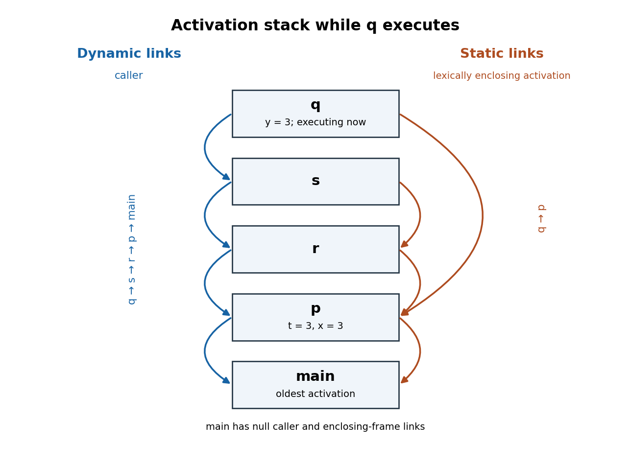

Figure 1.
The call stack during `q`, with dynamic links on the left and static links on the right; arrows point to older stack frames
. **Details**.

The dynamic chain is

q ⟶ s ⟶ r ⟶ p ⟶ main .

The individual static links are

q ⟶ p, s ⟶ r, r ⟶ p, p ⟶ main .

main has no enclosing procedure; its links can be null. The p stack frame contains t=3 and x=3, and the q stack frame contains y=3. Return addresses are code addresses, not links to another stack frame. In particular, q returns dynamically to s while obtaining x statically from p.

b

Solution

We specify a small stack machine instruction convention because the paper does not prescribe instruction spellings or numeric stack frame offsets. PUSHFP pushes the current frame pointer. LOAD k replaces a stack-top frame address by the value at fixed offset k in that frame. Let SL be the static link offset, X the offset of p's x, and Y the offset of q's parameter y. ADD pops two integers and pushes their sum. RETVAL returns the stack-top value, removes the current activation and restores the caller through the usual calling convention.

PUSHFP       ; address of q's frame
LOAD SL      ; q's static link: address of p's frame
LOAD X       ; value of p.x
PUSHFP       ; address of q's frame, above x
LOAD Y       ; q's local parameter y
ADD          ; x + y
RETVAL       ; return the sum to s

One static link traversal suffices for x, despite three intervening calls in the dynamic chain. y is local to q. In this execution the two loads produce

3

and

3

, so the returned integer is

6

c

Solution

Continue the instruction convention above. The current stack frame is now s's. Its static chain passes through r to p; q is declared directly inside p, so the new q activation must receive a static link to that same p stack frame. Let T be the offset of p's parameter t.

Define CALL q,1 to expect, above the pre-existing evaluation stack, the static link for q followed by its one argument. It consumes these, creates q's stack frame with its dynamic link pointing to the current s activation, and leaves one return value when q returns. This explicit convention avoids dependence on a particular real instruction set architecture.

PUSHFP       ; s
LOAD SL      ; r
LOAD SL      ; p, the required static parent of q
DUP          ; preserve p for CALL while also using it to read t
LOAD T       ; replace the duplicate p address by p.t
CALL q,1     ; q(p.t), with static parent p and dynamic caller s
RETVAL       ; return q's result from s to r

Immediately before CALL, the evaluation stack ends in p-frame, 3. Two static link traversals find both the argument's environment and the environment to pass to q. In terms of the hidden argument and ordinary argument,

SL_{q} = frame_{p}, y = t = 3.

An implementation that places the hidden static link after the ordinary argument could use a different ordering of these same operations.

d

Solution

Use mathematical induction on the sequence of call and return events. The invariant concerns the static chain of the currently executing activation: every stack frame on that chain is the most recent surviving activation of the procedure it represents. It need not hold for the saved chain of an arbitrary suspended caller while a recursive callee is running.

Initially only main is active, so the claim holds. Suppose it holds just before a direct call to a procedure

R

, whose lexical parent is

P

. Without procedural parameters, visibility of

R

means that its declaration lies in the current procedure or in a lexically enclosing procedure. Therefore the activation of

P

needed for the call is on the caller's static chain. By the induction hypothesis, it is the newest surviving activation of

P

Create a new activation of

R

whose static link points to this

P

activation. The inherited chain is a suffix of the caller's chain, so its stack frames still represent the newest surviving activations of their procedures. Adding

R

does not make any of those inherited activations out of date:

R

cannot be its own lexical ancestor. The new

R

activation itself is plainly the newest activation of

R

. This covers recursive calls too: an older activation of

R

may survive on the dynamic chain, but is absent from the new activation's static chain.

On return, the callee and every call it made have finished. The caller's saved stack frame and static chain are restored. Any temporarily newer activation of a procedure represented on that chain has returned, so each restored activation is again the most recent surviving one. Thus return preserves the invariant as well.

The claim holds for the executing procedure's static chain throughout every execution using direct calls under lexical scope. Equivalently, writing

P_{F}

for the procedure represented by a stack frame

F

F \in staticChain_{executing} ⟹ F = newestSurviving (P_{F}) .

e

Solution

Searching the dynamic chain would require identifying the procedure associated with each visited stack frame. More seriously, the search length is bounded by the number

h

of active calls, not by lexical nesting depth. Recursion in procedures unrelated to the desired enclosing declaration can make

h

arbitrarily large. Thus a single nonlocal variable access can take

O (h)

time complexity, whereas a conventional static chain access needs only

d

traversals for lexical distance

d

Instead give each procedure

P

a known global pointer cell current[P]. On entry to

P

, save its previous value in the new stack frame and set current[P] to the new frame pointer. On return, restore the saved value. A nonlocal variable declared in

P

is then loaded using current[P] and its known frame offset. The proof in part (d) justifies that lookup in the absence of procedural parameters. This is a procedure-indexed version of a display for lexical scope; a conventional display for lexical scope can instead use lexical levels as indices.

With

m

procedures and

h

active calls, the procedure-indexed table needs

O (m)

additional global words and one saved previous pointer per active stack frame, hence

O (h)

activation storage. The saved word can replace the conventional per-frame static link if that link is no longer needed. A conventional static chain has one pointer per active stack frame and no such

m

-entry table. Both schemes retain ordinary dynamic links and return information.

The table gives constant-time nonlocal access and constant-time save/restore work on each entry/return, independently of lexical distance. Conventional static chain access costs

O (d)

per access, and establishing the callee's static link may also require following an appropriate portion of the caller's chain. For a fixed program

d

is statically bounded, but it still affects generated instruction counts. These costs assume constant-cost pointer operations and omit shared ordinary call overhead. For the procedure-indexed table,

T_{access} = O (1), T_{entry/return} = O (1), S_{environment} = O (m + h) .

f

Solution

No: a procedural parameter can carry an older lexical environment past a newer recursive activation. Here is typed, Pascal-like pseudocode; a function-valued parameter is represented by a programming closure, comprising code and its defining environment.

procedure dummy(): integer;
begin return 0 end;

procedure P(n: integer; f: procedure(): integer): integer;
    var x: integer;
    procedure Q(): integer;
    begin return x end;
begin
    x := n;
    if n = 1 then return P(2, Q)
             else return f()
end;

begin print P(1, dummy) end.

Call the first P activation

P_{1}

. It sets its own x to

1

and passes the programming closure

(Q, P_{1})

into a recursive activation

P_{2}

. That activation sets its own x to

2

and calls its parameter f. The resulting activation of Q has its static link pointing to

P_{1}

, because that is where the passed procedure was defined. Its dynamic link points to

P_{2}

, because that is where it was called.

During this call the dynamic chain contains Q, P2, P1, main, while Q's static chain contains Q, P1, main. The newest surviving activation of P is

P_{2}

, but the static chain deliberately uses

P_{1}

. Correct lexical scope therefore prints

1

; blindly consulting current[P] would produce

2

. Both enclosing activations remain alive, so no issue of a returned procedure or dangling pointer is involved.

The failed step in part (d) is precisely the assumption that the callee's lexical environment is a suffix of the direct caller's static chain. A passed programming closure can specify a different, still surviving environment. An implementation supporting such calls must preserve that environment; a table implementation requires additional environment installation and restoration rather than merely consulting newest activations.

3

a

Solution

Use the following explicit tree notation for the intermediate representation. C(k) is a constant, R(r) a processor register, M(e) a word load from memory address e, ADD addition, and SHL(e,2) a left shift by two bits. MOVE(destination,source) assigns either a processor register or the computer memory word designated by M. Parentheses show complete tree structure, so these displays specify trees rather than already shared Directed acyclic graphs.

Let

A

be the constant base memory address of the global array a, and

I

the constant offset of local i from the frame pointer fp. Each integer occupies four bytes, and array indices are zero-based; a fixed nonzero lower bound can instead be absorbed into

A

. Local t is represented by R(t). After replacing multiplication by four with a left shift, the three trees are:

MOVE(R(t),
     M(ADD(C(A),
           SHL(M(ADD(C(A),
                     SHL(M(ADD(R(fp),C(I))),2))),2))))

MOVE(M(ADD(C(A),
           SHL(M(ADD(C(A),
                     SHL(M(ADD(R(fp),C(I))),2))),2))),
     M(ADD(C(A),SHL(M(ADD(R(fp),C(I))),2))))

MOVE(M(ADD(C(A),SHL(M(ADD(R(fp),C(I))),2))),
     R(t))

Every M(ADD(R(fp),C(I))) loads i; the next enclosing M loads a[i]; the outermost M in the first tree loads a[a[i]]. Each array index is converted to a byte offset by a left shift of two bits. The address rule used in all three trees is

addr (a [k]) = A + (k ≪ 2) = A + 4 k .

The source language's array bounds checks are omitted as requested.

b

Solution

The useful repeated program expressions, nested inside one another, are the memory address of a[i], its value, and the memory address of a[a[i]]. Materialize each maximal reusable tree at the level at which it is shared, using fresh temporary variables u, v, and w:

MOVE(R(u), ADD(C(A),SHL(M(ADD(R(fp),C(I))),2)))
MOVE(R(v), M(R(u)))
MOVE(R(w), ADD(C(A),SHL(R(v),2)))
MOVE(R(t), M(R(w)))
MOVE(M(R(w)), R(v))
MOVE(M(R(u)), R(t))

Thus u is a saved memory address, v the old integer value of a[i], w the second saved memory address, and t the old value at that second location. The two large address trees occur both in loads and as store destinations. After extracting them, the repeated load of a[i] inside the second address and as the middle assignment's source becomes v. Extracting every smaller nested tree again would add no benefit.

The relevant alias analysis facts are that local i does not occupy any location written through global a, that frame pointer fp and base

A

stay fixed, and that t,u,v,w are distinct processor registers or otherwise nonoverlapping temporary variables. There are no intervening calls, volatile memory accesses, or concurrent changes. Under these assumptions, loading i once remains valid even across the array stores. Before the middle store, no array location has yet changed, so both its target memory address and its source value can be computed and saved earlier.

No assumption that the two array locations are distinct is required. The middle store may change a[i] when its target coincides with it, but v is not loaded again afterwards: only the saved address u is needed for the final store. It would be unsound to retain an arbitrary array load across an aliasing store and then treat it as the new contents; that is not what these trees do.

For a language with a true global array, a distinct local variable, and no arbitrary means of fabricating pointers to unrelated storage, these facts follow simply from declarations and the stack frame layout. Accesses must denote valid array elements. In an unrestricted low-level language with overlapping storage, arbitrary pointer arithmetic or unchecked out-of-range accesses, that conclusion requires extra guarantees. Omitting emitted array bounds checks does not itself prove that all memory addresses are valid. If

M

denotes a word load, the saved quantities are

u = A + (i ≪ 2), v = M (u), w = A + (v ≪ 2) .

c

Solution

Here is a literal instruction selection for the trees in part (b), with the temporary variables allocated to processor registers. MOV r,#k loads an arbitrary constant in one instruction. LD and ST load and store one four-byte word; [r] denotes zero-offset access. LSL is a left shift. We use conventional base-plus-immediate access for the fixed local offset I.

MOV  rb, #A
LD   ri, [fp + I]
LSL  ru, ri, #2
ADD  ru, rb, ru
LD   rv, [ru]
LSL  rw, rv, #2
ADD  rw, rb, rw
LD   rt, [rw]
ST   rv, [rw]
ST   rt, [ru]

The first four instructions construct u, the fifth obtains v, the next two construct w, and the last three perform the remaining load and the two stores. Each destructive update of ru or rw reuses a processor register whose previous value is no longer needed. We assume enough processor registers to avoid a register spill.

If the target offers only the explicitly mentioned two-register register-offset addressing and lacks base-plus-immediate access, replace the one local load by MOV rk,#I; LD ri,[fp+rk]; all other conclusions are unchanged. A zero processor register or a zero-offset load supplies the notation [ru] and [rw] as usual. This direct translation takes ten instructions with immediate local addressing, or eleven with the stated replacement. Thus

N_{direct} = 10 (11 with the register-only local load) .

These are instruction counts for the specified abstract target, not measured execution times.

d

Solution

The target's register-offset addressing already performs the addition of the array base and a scaled index as part of each load or store. Materializing a maximal common address expression into a processor register introduces an explicit ADD that this addressing mode could have supplied. Here the extra address temporary variables save no arithmetic that the memory instructions need to perform separately.

Instead keep the scaled indices, share the loaded old value of a[i], and fold the base addition into each memory operand:

MOV  rb, #A
LD   ri, [fp + I]
LSL  rj, ri, #2
LD   rv, [rb + rj]
LSL  rk, rv, #2
LD   rt, [rb + rk]
ST   rv, [rb + rk]
ST   rt, [rb + rj]

rj remains the original index's byte offset, rv is its old element, and rk remains the second element's byte offset. Both stores use those saved offsets. Folding address additions into the memory instructions removes two instructions, reducing ten to eight, or eleven to nine if the local load requires the alternative sequence described in part (c). Therefore

N_{folded} = N_{direct} - 2 = 8 (or 9) .

This illustrates why common subexpression elimination must interact with instruction selection: a larger repeated tree is not automatically a better value to materialize. A useful refinement retains common scaled-index trees, or propagates the address addition trees back into their memory uses. The calculation establishes an instruction-count improvement under the stated instruction set architecture; scheduling and actual timing depend on further machine details.

e

Solution

The source rewrite already saves the old a[i] in register-allocated t. Denote the original integer index by

i_{0}

, its original element by

j = a [i_{0}]

, and the original element there by

k = a [j]

. The second fragment first sets t=j, then writes

k

to a[i0], and finally writes

j

to a[j]. Thus it performs the same intended swap without needing to recompute the second memory address from a possibly modified array element.

For completeness, the first fragment is also correct when the two locations might alias. If

j \neq = i_{0}

, its middle store changes only a[j], so the final a[i] still denotes the first location. If

j = i_{0}

, then

k = a [j] = a [i_{0}] = j = i_{0}

, and the supposed swap is a no-op in both fragments. There is no need to assume distinct locations.

For the second fragment, common subexpression elimination of maximal addresses gives, using z for the second address:

MOVE(R(u), ADD(C(A),SHL(M(ADD(R(fp),C(I))),2)))
MOVE(R(t), M(R(u)))
MOVE(R(z), ADD(C(A),SHL(R(t),2)))
MOVE(M(R(u)), M(R(z)))
MOVE(M(R(z)), R(t))

The nested memory-to-memory assignment requires an additional scratch processor register rv on a reduced instruction set computer. A direct translation is therefore:

MOV  rb, #A
LD   ri, [fp + I]
LSL  ru, ri, #2
ADD  ru, rb, ru
LD   rt, [ru]
LSL  rz, rt, #2
ADD  rz, rb, rz
LD   rv, [rz]
ST   rv, [ru]
ST   rt, [rz]

The same compiler need not produce any better code: this has the same ten-instruction count as part (c). It still performs two element loads, two element stores, two shifts and two separately materialized address additions, plus the base and local-index setup. The processor register roles and store order differ, but the work is the same. The corresponding folding of register-offset addressing removes both ADD instructions here too, yielding the same eight-instruction count as part (d).

The key alias analysis advantage available in both fragments is that i remains unchanged by the array stores. In the second fragment, t is also unchanged after its first assignment because it lives in a processor register. Its name alone does not produce a further saving beyond what the first fragment's common subexpression elimination already achieves. Exact instruction selection is not uniquely prescribed by the paper; these explicit translations demonstrate why the claimed source-level efficiency advantage does not follow:

N_{second} = N_{first} = 10 (both reduce to 8 after address folding) .

Computational complexity (A12071W1)

Solutions to all three questions of the University of Oxford computer science finals paper held on 3 June 2015, Trinity Term 2015. The printed cover gives paper code A12071W1. Questions 2 and 3 are marked corrected in the source.^[ref]

The solutions use the original printed notation; the integer parity convention needed in Question 3(e) is stated there explicitly.

1

a

Solution

Exactly the regular languages. A read-only-from-left Turing acceptor has only its current control state as usable memory: it never changes a tape symbol, and its head never returns to an earlier cell. This is the behaviour of a deterministic finite automaton while it reads the input.

To make the correspondence precise, retain the control states and the transitions on the input alphabet. Replace accepting and rejecting halts by absorbing states, so that halting before the end of a word over an alphabet has the same effect on every continuation. For each remaining state

q

, follow the transitions on blank symbols and mark

q

accepting in the deterministic finite automaton exactly when this blank-only continuation eventually accepts. This marking is a finite calculation: either a halting state is reached or a state repeats, after which the blank-only run loops. The resulting deterministic finite automaton accepts exactly the same formal language as the read-only-from-left Turing acceptor. If the latter is a decider, the blank-only run from every reachable end-of-input state halts.

Conversely, simulate any deterministic finite automaton by a read-only-from-left Turing acceptor, using its state transitions while reading the input. At the first blank symbol, halt and accept or reject according to the current deterministic finite automaton state. This machine halts on every input and decides the required regular language.

ROFL-decidable languages = regular languages .

b

Solution

Rice's theorem, in its formal language version, says: every nontrivial property of the computably enumerable language accepted by a Turing machine has an undecidable set of machine descriptions. Here nontrivial means that some computably enumerable language has the property and some does not. The property must be an extensional property of programs: any two Turing machines accepting the same formal language must agree about it. It need not be a property of all formal languages, including those no Turing machine accepts.

Let

P

be such a property and write

I_{P} = {enc (N) : L (N) \in P} .

We prove the theorem by a many-one reduction from the halting problem. First suppose the empty language is not in

P

. Nontriviality provides a fixed Turing machine

B

with

L (B) \in P

. Given a Turing machine

M

and a word over an alphabet

w

, effectively construct a Turing machine

N_{M, w}

which, on input

x

, first simulates

M

w

. If that simulation ever halts, it simulates

B

x

and accepts precisely when

B

accepts. If the first simulation never halts, it never accepts

x

The Turing machine encoding of

N_{M, w}

is computable from those of

M, w

: the description merely embeds

M, w

and the fixed simulator for

B

. Constructing it does not require predicting whether

M

halts. Its accepted formal language is

L (N_{M, w}) = {L (B), \emptyset, M halts on w, M does not halt on w .

Consequently

M halts on w ⟺ enc (N_{M, w}) \in I_{P} .

A decider for

I_{P}

would therefore decide the halting problem, a contradiction. Invalid descriptions can be mapped to a fixed description of a machine accepting the empty language, if the many-one reduction is formulated on all strings.

If the empty language does belong to

P

, apply the preceding argument to the opposite property, within the computably enumerable languages. This opposite property is still nontrivial and excludes the empty language. A hypothetical decider for

I_{P}

would decide the opposite property's index set by first rejecting malformed Turing machine encodings and otherwise reversing its answer. The opposite property is undecidable by the first case, giving the required contradiction in this case too.

I_{P} is undecidable for every nontrivial extensional P .

c

Solution

For example, take

L = {enc (M) : M has an even number of states} .

This is a decidable language: check that the input is a valid Turing machine encoding, count its declared states, and test the count's integer parity. There are Turing machines with even state counts and Turing machines with odd state counts, so the formal language contains some but not all valid descriptions.

There is no contradiction with Rice's theorem because this is a syntactic property of the description. Add one unreachable state to a Turing machine, assigning any permitted transitions to it. The accepted formal language is unchanged, while the integer parity of the state count changes. Thus the property is not an extensional property of programs, which is an essential hypothesis of Rice's theorem.

d

Solution

$L_{ℓ 3}$ is undecidable. The condition depends only on the accepted formal language. It holds for a Turing machine accepting the empty language, and fails for a Turing machine accepting the singleton

{aaaa}

, where

a

is an alphabet symbol. It is therefore a nontrivial extensional property of programs, and Rice's theorem applies. In particular, the condition does not assert that the machine halts on every input; nonacceptance of long words over an alphabet may result from rejection or from an infinite computation.

$L_{1 T}$ is a decidable language: it consists of every valid Turing machine encoding. Every multitape Turing machine has an equivalent single-tape Turing machine. To see this, represent the finitely used portions of its tapes on one tape, separated by delimiters, and mark each simulated head position. To simulate one step, scan these portions to read the marked symbols, retain this fixed number of symbols and the control state in finite control, and scan again to update the symbols and head marks. Extend a represented portion with a blank cell when necessary. Each simulated step takes finitely many real steps.

The single-tape Turing machine accepts exactly when the simulated multitape Turing machine accepts; infinite computations remain infinite. The simulation may increase time complexity, but the question only asks about accepted formal languages. Hence a decider simply checks the syntax of the Turing machine encoding and accepts every valid description. Rice's theorem does not make this property undecidable, because the property is true of every computably enumerable language and is therefore trivial in the theorem's sense.

L_{ℓ 3} is undecidable; L_{1 T} is decidable .

e

Solution

The clique decision problem is a decidable language: on a valid finite graph and an integer

k

, reject if

k

exceeds the number of vertices, and otherwise examine all

k

-element subsets of vertices, accepting if one is a clique. Each candidate can be checked by examining all its pairs of distinct vertices. This finite search gives at least one Turing machine deciding the problem, without any claim of polynomial time.

By well-ordering of the natural numbers, there is a least state count

n_{0}

among Turing machines deciding the clique decision problem. For every

n \geq n_{0}

, add

n - n_{0}

unreachable states to a machine with

n_{0}

states. Its behaviour on every input is unchanged, and it has exactly

n

states. For

n < n_{0}

there is no such machine, by minimality. Thus

L_{cliqueTM} = {enc (n) : n \geq n_{0}} .

A Turing machine with the fixed constant

n_{0}

in its description decides this threshold language by validating the input and comparing its value with

n_{0}

. The argument proves the existence of a decider; it does not compute the smallest possible clique decision problem decider. There is no need to search through machine descriptions and attempt to certify their behaviour on every input.

f

Solution

Let

V

be the decidable language of syntactically valid descriptions

enc (M) ## w

. Then

L_{H} \dot{\cup} L_{NH} = V, \overline{L_{H}} = L_{NH} \dot{\cup} (Σ^{*} ∖ V) .

Here the complement of a set on the left is taken in all words over an alphabet, while the non-halting problem only has valid machine-and-input descriptions as instances. Any malformed description belongs to $\overline{L_{H}}$ but not to $L_{NH}$ . For example, the empty word has no separating ##, so cannot be a valid instance under the displayed encoding.

Fix valid descriptions

h

and

ℓ

of, respectively, an immediately halting Turing machine on the empty word and a Turing machine looping forever on the empty word. Then

h \in L_{H}, ℓ \in L_{NH} .

For the first many-one reduction, use the total computable function

f (x) = {x, ℓ, x \in V, x \in / V .

For a valid input, nonmembership in

L_{H}

is exactly membership in

L_{NH}

, so retaining it is correct. Every invalid input is a yes-instance of

\overline{L_{H}}

, and

f

sends it to the fixed yes-instance

ℓ

. Therefore

x \in \overline{L_{H}}

if and only if

f (x) \in L_{NH}

For the reverse many-one reduction, use

g (x) = {x, h, x \in V, x \in / V .

The equivalence again holds on valid inputs. Invalid inputs are no-instances of

L_{NH}

, and

h

is a no-instance of

\overline{L_{H}}

. Syntax checking terminates, so

g

is also a total computable function. We have proved

\overline{L_{H}} \leq_{m} L_{NH} and L_{NH} \leq_{m} \overline{L_{H}} .

2

a

Solution

Writing

PTime

as P and

co - PTime

as co-P, the known relationships among the four complexity classes are

P = co - P, P \subseteq NP, P \subseteq co - NP .

The equality supplies both inclusions between P and co-P, and it also gives co-P

\subseteq

NP and co-P

\subseteq

co-NP.

For the equality, a deterministic polynomial-time algorithm halts on every input; interchange its accepting and rejecting outcomes to decide the complement of a set in the same polynomial time. For P

\subseteq

NP, a Nondeterministic Turing machine can simply make no choices and follow the deterministic computation. Finally, if

A \in P

, then

\overline{A} \in P \subseteq NP

, whence

A \in co - NP

by the definition of co-NP.

Neither NP

\subseteq

co-NP nor co-NP

\subseteq

NP is known; either would imply equality by taking complements. Nor is either inclusion of P into NP or co-NP known to be strict. These unresolved relationships must not be presented as strict separations.

b

Solution

The linear speedup theorem concerns multitape Turing machines whose finite control and tape alphabet may change. Formally, for

k > 1

, if a deterministic

k

-tape Turing machine decides

A

within

T (n)

steps on every input of length

n

, then for every constant

c > 0

there is a deterministic

k

-tape Turing machine deciding the same formal language with

T_{c} (n) \leq \frac{T ( n )}{c} + n + O (1) .

The additive constant is independent of

n

; in the usual normalized formulation the bound is

T (n) / c + n + 2

, with the integer-rounding convention absorbed in the constant.^[ref]

The construction packs a fixed number of old tape symbols into each new symbol and uses a larger finite control to simulate blocks of old steps. Initial input packing explains the additive linear term. If

T (n) / n \to \infty

, choosing a larger constant

c

makes the total asymptotic time complexity an arbitrarily small constant multiple of

T (n)

It does not promise arbitrary speed increases on fixed hardware. Larger packed symbols and transition tables cease to be single constant-cost hardware operations without limit. The theorem also retains the input-reading overhead. It is a statement about changing the abstract machine description and primitive operations, rather than an unlimited implementation optimization on one processor.

c

Solution

Let

A \in NP

, accepted by a fixed Nondeterministic Turing machine

M

in at most

p (n)

steps on every computation branch, for a polynomial

p

. Since the transition relation is finite, there is a fixed constant

b \geq 2

bounding the number of choices at any step. Every branch can be specified by a word over an alphabet of length

p (n)

over a

b

-symbol choice alphabet, padding unused choices after halting.

A deterministic Turing machine enumerates all

b^{p (n)}

such choice sequences and simulates the corresponding branches for at most

p (n)

steps each. It accepts if some simulation accepts, and rejects after all have failed. Every possible accepting branch is included, and the time cutoff guarantees termination even on invalid choice sequences. A standard direct simulation has only polynomial overhead per branch, giving

b^{p (n)} p (n)^{O (1)} = 2^{O (p (n) + l o g (p (n) + 1))} \leq 2^{q (n)}

for a suitable polynomial

q

. This is a deterministic exponential time bound. Therefore

NP \subseteq EXPTIME .

Here EXPTIME means the union of deterministic time bounds

2^{n^{d}}

over fixed positive integers

d

, allowing the usual constant factors and finitely many small inputs.

d

Solution

Entail is co-NP-complete under polynomial-time many-one reductions. For valid propositional formulas, semantic entailment holds exactly when the logical conjunction of the premise and the conclusion's logical negation is an unsatisfiable Boolean formula:

φ ⊨ ψ ⟺ φ \land \neg ψ is unsatisfiable .

A counterexample to semantic entailment is a Boolean valuation making

φ

true and

ψ

false. Guessing one bit for each distinct Boolean variable and evaluating both propositional formulas is a polynomial-time algorithm. Thus the complement of Entail belongs to NP. Malformed descriptions, also in that complement, can be accepted after a deterministic syntax check. Hence Entail belongs to co-NP as a formal language over all strings.

For hardness, the unsatisfiable Boolean formula problem is co-NP-hard: if

A \in co - NP

, then

\overline{A} \in NP

, and the permitted NP-hardness of SAT supplies a polynomial-time many-one reduction

r

with

x \in \overline{A} ⟺ r (x) \in SAT .

We may ensure

r (x)

is always a valid propositional formula, replacing any malformed output by a fixed contradiction. It follows that

x \in A

exactly when

r (x)

is unsatisfiable. This justifies using the unsatisfiability problem as a hardness source without an extra assumption.

Map a valid propositional formula

θ

f (θ) = ⟨ θ, p \land \neg p ⟩,

where

p

is a fixed Boolean variable. The second propositional formula is false under every Boolean valuation. Consequently it is entailed by

θ

precisely when no Boolean valuation satisfies

θ

. Thus

θ unsatisfiable ⟺ f (θ) \in Entail .

The output has only constant additional length and is computable in polynomial time. If the source unsatisfiability language rejects malformed strings, map them to the fixed no-instance

⟨ p, p \land \neg p ⟩

. This completes a total polynomial-time many-one reduction and proves the claimed co-NP-completeness.

Entail is co-NP-complete .

e

Solution

The clique decision problem belongs to NP. First reject

k > ∣ V (G) ∣

. Otherwise a complexity certificate lists

k

distinct vertices. Check distinctness and test that each of the

(2 k)

pairs is an edge. Under a conventional explicit graph encoding, the complexity certificate length and verification time complexity are polynomial in the input length. The early rejection is relevant when

k

is given in the binary numeral system.

For NP-hardness, first transform a SAT instance into an equisatisfiable conjunctive normal form

F = C_{1} \land \dots \land C_{m}

of polynomial size using a Tseitin transformation. This step avoids the possibly exponential increase caused by distributing arbitrary Boolean formulas into conjunctive normal form. Introduce a fresh Boolean variable for each subformula, constrain it to have the connective's truth value using a constant number of Boolean clauses, and require the top variable to be true. A Boolean valuation of the original Boolean variables satisfies the original Boolean formula exactly when it extends to a satisfying assignment of these constraints.

Create one vertex for each occurrence of a Boolean literal in each Boolean clause. Join two such vertices by an edge exactly when they belong to different Boolean clauses and their Boolean literals are not a variable and its logical negation. Set

k = m

. There are at most as many vertices as Boolean literal occurrences and at most quadratically many edges, so this construction takes polynomial time.

F

has a satisfying assignment, choose one true Boolean literal occurrence from each Boolean clause. No two selected Boolean literals are contradictory, so their

m

vertices form a clique. Conversely, an

m

-clique contains at most one vertex from each Boolean clause, because there are no edges within a Boolean clause. It therefore selects exactly one occurrence from each of the

m

Boolean clauses. The selected Boolean literals are pairwise noncontradictory, so assign their Boolean variables the indicated truth values and assign any other Boolean variables arbitrarily. This Boolean valuation satisfies every Boolean clause.

An empty Boolean clause gives no vertex in its group, correctly preventing an

m

-clique. An empty logical conjunction can instead be mapped to a fixed yes-instance, avoiding any convention about

k = 0

. Malformed SAT descriptions can be mapped to a fixed no-instance. We have proved

F satisfiable ⟺ ⟨ G_{F}, m ⟩ \in Clique, Clique is NP-complete .

f

Solution

To establish strong NP-completeness, use an explicit adjacency matrix encoding for a finite simple graph, with enough length information to recover its number

N

of vertices. Let

bin (k)

be the canonical binary numeral system representation of the nonnegative integer

k

. Define

L_{Clique} = {⟨ enc (G), bin (k)⟩ : G has a clique of size k},

and, using the unary numeral system for

k

L_{u Clique} = {⟨ enc (G), 1^{k} ⟩ : G has a clique of size k} .

The surrounding pairing syntax delimits the two components, so the empty unary field can encode

k = 0

if zero is included in the convention for natural numbers. Malformed descriptions are excluded from both formal languages.

Fix a unary no-instance

u_{0}

, for example one isolated vertex with requested size

2

. The polynomial-time many-one reduction is

f (⟨ enc (G), bin (k)⟩) = {⟨ enc (G), 1^{k} ⟩, u_{0}, 0 \leq k \leq N, k > N .

Map malformed inputs to

u_{0}

too. When

k \leq N

, only the numerical representation changes, so the existence of a

k

-clique is unchanged. When

k > N

, the original instance is false, since a subset of vertices cannot be larger than the whole vertex set;

u_{0}

is false as required.

The important size bound is

k \leq N

in the branch that writes

1^{k}

. The original explicit graph description already has length at least

N

, so the output has polynomial length and can be written in polynomial time. If a huge binary numeral system value

k

is supplied, compare it with

N

using its digit length and, when needed, a digit comparison; do not first allocate or print

k

symbols. Merely replacing an unrestricted binary

k

1^{k}

would not be a valid polynomial-time reduction.

Thus

L_{Clique} \leq_{p} L_{u Clique}

. The unary version is in NP by the same clique complexity certificate verification, and is NP-hard by this polynomial-time many-one reduction and part (e). Therefore

Clique is strongly NP-complete .

This conclusion uses the conventional explicit graph encoding; a succinct circuit description of a graph would be a different input representation and a different problem.

3

a

Solution

Use Turing machines with a two-way read-only input tape, bounded by endmarkers, and a fixed finite number of read-write work tapes over a fixed finite alphabet. Work-tape cells count towards space complexity; the read-only input does not. For input length

n

, use

O (lo g (n + 2))

to include the small-length cases.

$Logspace$ , or L, is the class of formal languages decided by a deterministic such machine using at most $c lo g (n + 2)$ work-tape cells for some fixed constant $c$ . It must halt on every input and accept exactly the members.

$NLogspace$ , or NL, is the class of formal languages accepted by a Nondeterministic Turing machine with the same work-space bound on every computation branch. An input is accepted if and only if at least one branch accepts. One may require all branches to halt: the configuration graph has only a polynomial number of vertices, so a logarithmic space counter can stop any branch that has taken more steps than that bound. If an accepting computation exists, one exists with no repeated Turing machine configuration, so this convention does not change the complexity class.

In standard space complexity notation,

L = DSPACE (O (lo g n)), NL = NSPACE (O (lo g n)) .

b

Solution

A logspace many-one reduction

A logspace transducer is a deterministic Turing machine with a read-only input tape,

O (lo g (n + 2))

read-write work space, and a write-only output tape. It emits symbols successively and cannot reread the output; that output is not charged as working memory. For a total function it must halt on every input. A logspace-computable function

f

is a total function whose output

f (x)

is produced by such a logspace transducer on input

x

A \leq_{m}^{l o g} B

is a logspace-computable function

f

such that

x \in A ⟺ f (x) \in B

for every string

x

. The logarithmic space bound permits a polynomial-length output, even when that output does not fit in work space. Indeed, a halting logspace transducer cannot repeat its state, input-head position and work-tape contents and head positions: the unreadable output cannot affect its subsequent behaviour. There are only a polynomial number of such internal Turing machine configurations, hence a polynomial bound on the number of steps and output symbols.

To prove a formal language

B

is NL-complete, first give an NL acceptance procedure for

B

. Then show every

A \in NL

has a logspace many-one reduction to

B

. Alternatively, reduce one already NL-complete formal language to

B

, using transitivity of logspace many-one reductions.

Transitivity requires logspace composition by recomputation, rather than storing the intermediate output. To compose

g

with

f

, simulate the logspace transducer for

g

with a virtual input

f (x)

. Retain its virtual input-head position in

O (lo g n)

bits. Whenever it asks for a symbol, rerun the logspace transducer for

f

from the beginning and count its output symbols until that position is reached. Since

∣ f (x) ∣

is polynomial in

n

, the simulated work space

O (lo g ∣ f (x) ∣)

and all output-position counters are

O (lo g n)

. Repeated runs reuse their storage. This proves closure under composition and explains why the hardness argument works.

c

Solution

Let a deterministic Turing machine

M

decide

A

with at most

s (n) = c lo g (n + 2)

work-tape cells. Fix an input

x

of length

n

. A Turing machine configuration is determined by the control state, the read-only input-head position, the work-tape contents, and the work-head positions. For one work tape with alphabet

Γ

, their number is bounded, up to harmless fixed factors, by

∣ Q ∣ (n + 2) (s (n) + 1) ∣Γ ∣^{s (n)} .

The factors respectively count the state, input-head position, work-head position and work-tape contents. With a fixed number

r

of work tapes, replace the last two factors by

(s (n) + 1)^{r} ∣Γ ∣^{rs (n)}

if each tape is allowed

s (n)

cells; this still gives a valid polynomial upper bound. Two-way work tapes only change fixed factors in the head-position bounds.

Since

∣Γ ∣^{c l o g_{2} (n + 2)} = (n + 2)^{c l o g_{2} ∣Γ∣},

there are at most

(n + 2)^{d}

Turing machine configurations for some constant

d

depending on

M

. If a deterministic computation repeats one of its Turing machine configurations on the fixed input, all subsequent steps repeat too, so it never halts. But

M

is a decider. It therefore halts before any repetition and takes at most a polynomial number of steps. The same Turing machine is consequently a polynomial-time algorithm, establishing

Logspace \subseteq PTime .

It would be incorrect to count just the work-tape contents and omit the read-only input-head position; that position is part of the Turing machine configuration even though the input itself is not charged as work space.

d

Solution

Directed reachability is NL-complete under logspace many-one reductions. For membership, let

N

be the number of vertices. Store a current vertex, initially

v

, and a counter initially zero. Accept immediately if the current vertex is

v^{'}

. Otherwise guess a next vertex, verify by scanning the input that the appropriate directed edge exists, move there and increment the counter. Reject a branch that has made

N - 1

steps without reaching

v^{'}

Whenever a directed walk reaches

v^{'}

, removing closed portions between repeated vertices produces a path in a graph with at most

N - 1

edges. Thus this bound preserves all yes-instances. The current and guessed vertices and the counter use

O (lo g N)

bits, while adjacency checks only need repeated read-only input scans. All branches halt, so directed reachability belongs to NL.

For hardness, let

A \in NL

and fix a Nondeterministic Turing machine

M

accepting

A

O (lo g n)

work space. On input

x

, construct its configuration graph

C_{x}

. A vertex is a possible Turing machine configuration within the fixed work-space bound. Put a directed edge

C \to D

exactly when one legal transition of

M

x

changes

C

into

D

. Take the initial Turing machine configuration as source, and add a fresh target

t

with an incoming edge from every accepting Turing machine configuration. Then

x \in A ⟺ the initial configuration reaches t in C_{x} .

There are only a polynomial number of Turing machine configurations, by the count used in part (c). More importantly, their encodings have length

O (lo g n)

. A logspace transducer can enumerate candidate encodings and pairs of candidate encodings with

O (lo g n)

bits of counters. For each pair, it checks the finite transition rule, the scanned input symbol and the local work-tape change using

O (lo g n)

work space. It emits the corresponding adjacency matrix entry or edge-list record. Invalid candidate encodings may be discarded or represented by isolated vertices.

The configuration graph is thus output by a logspace transducer, rather than stored in its work tapes. This supplies the required logspace many-one reduction from every

A \in NL

and proves NL-completeness.

Reachability is NL-complete .

e

Solution

The printed question calls the route a path in a graph and writes

p \subseteq E (G)

, without specifying whether repeated vertices are allowed.^[ref] Use the computational reachability convention that a permitted route is a directed walk: repeated vertices are allowed and length counts traversed edges with multiplicity. This matters for the integer parity restriction, because deleting a closed portion of odd length can change the integer parity. The proof below establishes the stated NL-completeness for this convention; it does not establish that claim for a simple path in a graph.

For membership of even-length directed reachability in NL, form the conceptual parity graph with vertex set

V (G) \times {0, 1}

and directed edges

(u, b) ⟶ (w, 1 - b) ⟺ (u, w) \in E (G) .

After a directed walk of length

j

from

(v, 0)

, the second coordinate equals

j mod 2

. Therefore there is an even-length directed walk from

v

v^{'}

G

exactly when

(v^{'}, 0)

is reachable from

(v, 0)

in this parity graph. It has

2 N

vertices. Guess successive edges while storing the original current vertex, one parity bit, and a counter bounded by

2 N - 1

. If the target pair is reachable, it has a simple path in a graph in this enlarged graph of at most

2 N - 1

edges. This is an NL procedure; the parity graph need not be materialized.

For NL-hardness, reduce directed reachability by subdividing each directed edge

(u, w)

with its own new vertex

a_{u w}

u ⟶ a_{u w} ⟶ w .

Retain

v, v^{'}

as the endpoints and add no other edges. Every original directed walk of length

j

becomes a directed walk of even length

2 j

. Conversely, a directed walk between original vertices in the new graph must alternate original and subdivision vertices. Compressing each two-edge segment recovers a directed walk in

G

. Hence

⟨ G, v, v^{'} ⟩ \in Reachability ⟺ ⟨ G^{'}, v, v^{'} ⟩ \in E - Reachability .

A logspace transducer enumerates the original edges, labels each new vertex by its edge endpoints or its position in the input, and emits its two replacement edges. All labels and counters take

O (lo g n)

bits, and the output is of polynomial size. Thus this is a logspace many-one reduction, proving

E - Reachability is NL-complete .