Put , the standard metric tensor on the unit sphere. From one has . The apparently divergent terms cancel:The metric tensor block has determinant , independently of . Its coefficients are real analytic, so this formula defines a regular Lorentzian metric onThe polar-coordinate degeneracies at the poles are handled by ordinary two-sphere charts. Thus is a coordinate singularity of the original chart and is crossed by this spacetime extension.
The inverse of the metric tensor block isThe normal covector has squared norm . ThereforeMore explicitly, the induced metric tensor is ; at zero its sole zero direction is . The coefficients are independent of , so is a Killing vector field. On ,Hence is both tangent and normal to this null hypersurface, proving it is a Killing horizon. The definition of surface gravity is on the Killing horizon, or equivalently . Since vanishes there while ,Thus this is a degenerate Killing horizon, and is an affine parameter on each of its null geodesics.
For a concrete horizon frequency comparison, fix the same angular position for a narrow high-frequency light beam and two freely falling radial observers. Work in geometric optics, with the beam's affinely transported wavevector tangent to the Killing horizon, . Here is constant because . Choose the observers as translates of one timelike geodesic by the isometry generated by , crossing at and . Give them the same positive Killing energy per unit rest mass, . At their crossings their normalized four-velocities havewhich satisfy . They can be realized by local geodesics with precisely these initial data. The measured angular frequency isTo connect this measurement to surface gravity, if with constant , affine transport of would give . For observers related by the same Killing vector field translation, agrees at the crossings, giving . Here there is no accumulated redshift along the Killing horizon for these equally prepared observers. Arbitrary observers with different four-velocities can still measure different frequencies through their different Killing energies.
First use the original null coordinates , . They obey , and the radial metric tensor becomesApply the given substitutions and . The identitiesgive the analytic extension of a spacetimeThe poles of the individual tangent and cotangent substitutions are now ordinary coordinate lines wherever . Set and . Allowing these coordinate functions to continue across every such line givesThis is the universal cover of two-dimensional anti-de Sitter spacetime of radius , times a two-sphere of radius : the simply connected Bertotti-Robinson spacetime. In defining this maximal analytic extension, ranges over the whole real line without periodic identification. A periodic identification would instead create closed timelike curves and would be an additional global choice.
For clarity, the original patch is embedded by the branches and . The inequality is equivalent on these branches to , so the original patch occupiesThe first spacetime extension in part (a) occupies the larger band , with . Its finite- Killing horizon is the interior line . The edges of that band are further regular Poincaré horizons; continuing through them produces the full conformal strip of two-dimensional anti-de Sitter spacetime.
The original coordinate has a smooth continuation throughout the strip:Consequently the complete set of zero-level Killing horizons isThese are two alternating families of parallel null lines; different families meet only at the excluded conformal boundaries, never inside the spacetime. The continuation of the original Killing vector field isThe field never vanishes in the interior, including on the Killing horizons.
To obtain the Penrose diagram, suppress the two-sphere and multiply by the conformal factor . The resulting radial metric tensor is , so the diagram is an infinitely tall strip of width , with null lines at 45 degrees and timelike edges . Generically,At the special edge points where the two families of Killing horizons end, the displayed formula is a limit and has no unique limiting value. Thus the infinity labels on the diagram refer to the open edge segments, not those vertices. Each interior point of the diagram represents a two-sphere of fixed radius ; neither edge is a centre where that two-sphere shrinks.
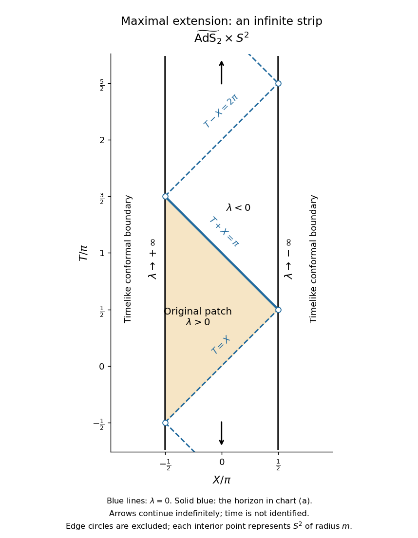
Penrose diagram of the maximal Bertotti-Robinson spacetime extension, with the original patch and all zero-level Killing horizons
. Details. 
Finally, these timelike edges are conformal boundaries, not omitted regular points of a further spacetime extension. One way to establish maximality is geodesic completeness. The two-dimensional anti-de Sitter spacetime factor embeds locally as in a flat space with metric signature . Along an affinely parametrized geodesic with constant , the ambient equation isIts oscillatory, linear or hyperbolic solutions for negative, zero or positive exist for all real affine parameters and lift to the universal cover. The two-sphere is also geodesically complete, and geodesics of the product split into geodesics of its factors. Hence is geodesically complete. A proper regular spacetime extension would furnish a geodesic reaching its boundary in finite affine parameter, contradicting that completeness. This proves that the displayed simply connected analytic spacetime is maximal.
Articles by others on the same topic
There are currently no matching articles.