Complete solutions to the three questions of the Part C General relativity II course of the University of Oxford paper, sat on 1 June 2021. Original released PDF, bundle pages 63–65; paper pages 1–3. The bundle filename says 2020, but the paper's cover explicitly says Trinity Term 2021. The metric signature is and the speed of light is set to one. All questions and both Roman-numbered parts of question 1(d) are covered.
Write , for the expansion scalar, for the four-acceleration, and for the spatial projector of a timelike congruence. The normalization of the four-velocity gives and . The product rule and metric compatibility give the covariant derivative of the perfect fluid in general relativity stress-energy tensor:Its tensor contraction with the four-velocity isand its projection with the spatial projector of a timelike congruence isThus stress-energy conservation implies the relativistic perfect-fluid energy equation and the relativistic Euler equation:Conversely, the two displayed equations set both projections of to zero. Since , they imply . This establishes equivalence, including points where , without dividing by that quantity.
Use stress-energy conservation and symmetry of the stress-energy tensor. The Killing equation for the Killing vector field then gives the stress-energy current from a Killing vector:Hence . The assumption of stress-energy conservation, supplied by the equations of motion in part (a), is essential; the Killing equation alone only eliminates the second term.
The sign of is unchanged by a nonzero rescaling of the timelike vector . Normalize it to a four-velocity and, after reversing its direction if necessary, write , where , and is the Lorentz factor. For the perfect fluid in general relativity,Taking requires . Allowing the Lorentz factor to become arbitrarily large requires ; otherwise sufficiently fast observers measure a negative value. Conversely, these two inequalities make both terms in the last expression nonnegative. Therefore the weak energy condition for a perfect fluid is exactlyProperty (1) is the weak energy condition: every physical observer measures nonnegative local energy density, namely for their normalized four-velocity . It allows negative pressure down to .
For relativistic dust, , the relativistic Euler equation gives . The nowhere-vanishing density therefore makes the four-acceleration zero: is a timelike geodesic vector field. Let be the differential one-form obtained by the musical isomorphism. Its exterior derivative satisfiesHere is the interior product. By hypersurface orthogonality and the Frobenius theorem, . Taking the interior product and using givesThus . By the Poincaré lemma, locally , and then . Choose spatial coordinate functions on one level set of and extend them constantly along the integral curves of a vector field , using its smooth flow. This constructs . Since ,The metric on the orthogonal complement of a timelike vector is positive-definite, so the synchronous coordinates for irrotational dust haveThis construction is local; crossing geodesics can prevent these synchronous coordinates from covering a larger region.
In the prescribed synchronous coordinates, the Christoffel symbols satisfyConsequently the four-acceleration of vanishes. For a spatial index , , so the spatial component of the relativistic Euler equation becomesOn a connected coordinate neighbourhood,A nonzero pressure is allowed, but its spatial gradient must vanish if the fluid's four-velocity follows these freely falling coordinate lines. No division by or is needed.
For the plane gravitational wave in linearized gravity, the chain rule gives . The Lorenz gauge in linearized gravity, called wave gauge in the paper, imposes zero divergence of the trace-reversed metric perturbation. HenceThe wave equation itself holds for any smooth profile of , because for the constant null vector .
Use the active sign convention for the linearized coordinate gauge transformation, . The paper's prescribed generator has precisely this sign; using the passive convention would require its negative. Direct partial differentiation givesThe middle terms cancel when the indices are symmetrized. ThereforeTo test both equations (3), put , the trace of the original metric perturbation. Since is a null vector, and its trace-reversed metric perturbation equals . Differentiating the result of part (a) givesIn the second identity, the term with is zero. ThusIn general does not satisfy (3). On an open interval of , both equations hold exactly when there: the first equation forces this for , and smoothness gives it at as well. A linearized coordinate gauge transformation preserves the linearized vacuum Einstein equations, but only a residual gauge symmetry of linearized gravity preserves the imposed Lorenz gauge in linearized gravity.
For an explicit failure, use the null coordinates of part (c) and take only nonzero. Then , the original field obeys (3), but gives and .
With and , the Minkowski metric and the specified null vector becomeThe Minkowski wave operator in null coordinates is . All components of the original metric perturbation still depend only on , since this coordinate change is linear. The result of part (a), differentiated once, readsIt follows that and . Taking the trace givesExpanding the scalar in these null coordinates therefore yieldswhere the coefficients are explicitlyThe quadratic transverse term is a harmonic quadratic plane-wave profile. In particular , and , consistently reproducing the failure of wave gauge in part (b).
Continue with the active sign convention for the linearized coordinate gauge transformation. Choose local functions of by integration so thatFor example, for any fixed one may takeA generator, specified as a covector with components in the null coordinates , isIndeed, with , the mixed components cancel:All components without a index vanish as well, andSince , only the component needs changing. ThusYes, satisfies both equations (3). Its trace is zero, gives zero divergence, and the harmonic quadratic plane-wave profile givesThe two surviving functions encode the two gravitational wave polarizations; constant and linear transverse terms have been removed by the explicit linearized coordinate gauge transformation.
Put , the standard metric tensor on the unit sphere. From one has . The apparently divergent terms cancel:The metric tensor block has determinant , independently of . Its coefficients are real analytic, so this formula defines a regular Lorentzian metric onThe polar-coordinate degeneracies at the poles are handled by ordinary two-sphere charts. Thus is a coordinate singularity of the original chart and is crossed by this spacetime extension.
The inverse of the metric tensor block isThe normal covector has squared norm . ThereforeMore explicitly, the induced metric tensor is ; at zero its sole zero direction is . The coefficients are independent of , so is a Killing vector field. On ,Hence is both tangent and normal to this null hypersurface, proving it is a Killing horizon. The definition of surface gravity is on the Killing horizon, or equivalently . Since vanishes there while ,Thus this is a degenerate Killing horizon, and is an affine parameter on each of its null geodesics.
For a concrete horizon frequency comparison, fix the same angular position for a narrow high-frequency light beam and two freely falling radial observers. Work in geometric optics, with the beam's affinely transported wavevector tangent to the Killing horizon, . Here is constant because . Choose the observers as translates of one timelike geodesic by the isometry generated by , crossing at and . Give them the same positive Killing energy per unit rest mass, . At their crossings their normalized four-velocities havewhich satisfy . They can be realized by local geodesics with precisely these initial data. The measured angular frequency isTo connect this measurement to surface gravity, if with constant , affine transport of would give . For observers related by the same Killing vector field translation, agrees at the crossings, giving . Here there is no accumulated redshift along the Killing horizon for these equally prepared observers. Arbitrary observers with different four-velocities can still measure different frequencies through their different Killing energies.
First use the original null coordinates , . They obey , and the radial metric tensor becomesApply the given substitutions and . The identitiesgive the analytic extension of a spacetimeThe poles of the individual tangent and cotangent substitutions are now ordinary coordinate lines wherever . Set and . Allowing these coordinate functions to continue across every such line givesThis is the universal cover of two-dimensional anti-de Sitter spacetime of radius , times a two-sphere of radius : the simply connected Bertotti-Robinson spacetime. In defining this maximal analytic extension, ranges over the whole real line without periodic identification. A periodic identification would instead create closed timelike curves and would be an additional global choice.
For clarity, the original patch is embedded by the branches and . The inequality is equivalent on these branches to , so the original patch occupiesThe first spacetime extension in part (a) occupies the larger band , with . Its finite- Killing horizon is the interior line . The edges of that band are further regular Poincaré horizons; continuing through them produces the full conformal strip of two-dimensional anti-de Sitter spacetime.
The original coordinate has a smooth continuation throughout the strip:Consequently the complete set of zero-level Killing horizons isThese are two alternating families of parallel null lines; different families meet only at the excluded conformal boundaries, never inside the spacetime. The continuation of the original Killing vector field isThe field never vanishes in the interior, including on the Killing horizons.
To obtain the Penrose diagram, suppress the two-sphere and multiply by the conformal factor . The resulting radial metric tensor is , so the diagram is an infinitely tall strip of width , with null lines at 45 degrees and timelike edges . Generically,At the special edge points where the two families of Killing horizons end, the displayed formula is a limit and has no unique limiting value. Thus the infinity labels on the diagram refer to the open edge segments, not those vertices. Each interior point of the diagram represents a two-sphere of fixed radius ; neither edge is a centre where that two-sphere shrinks.
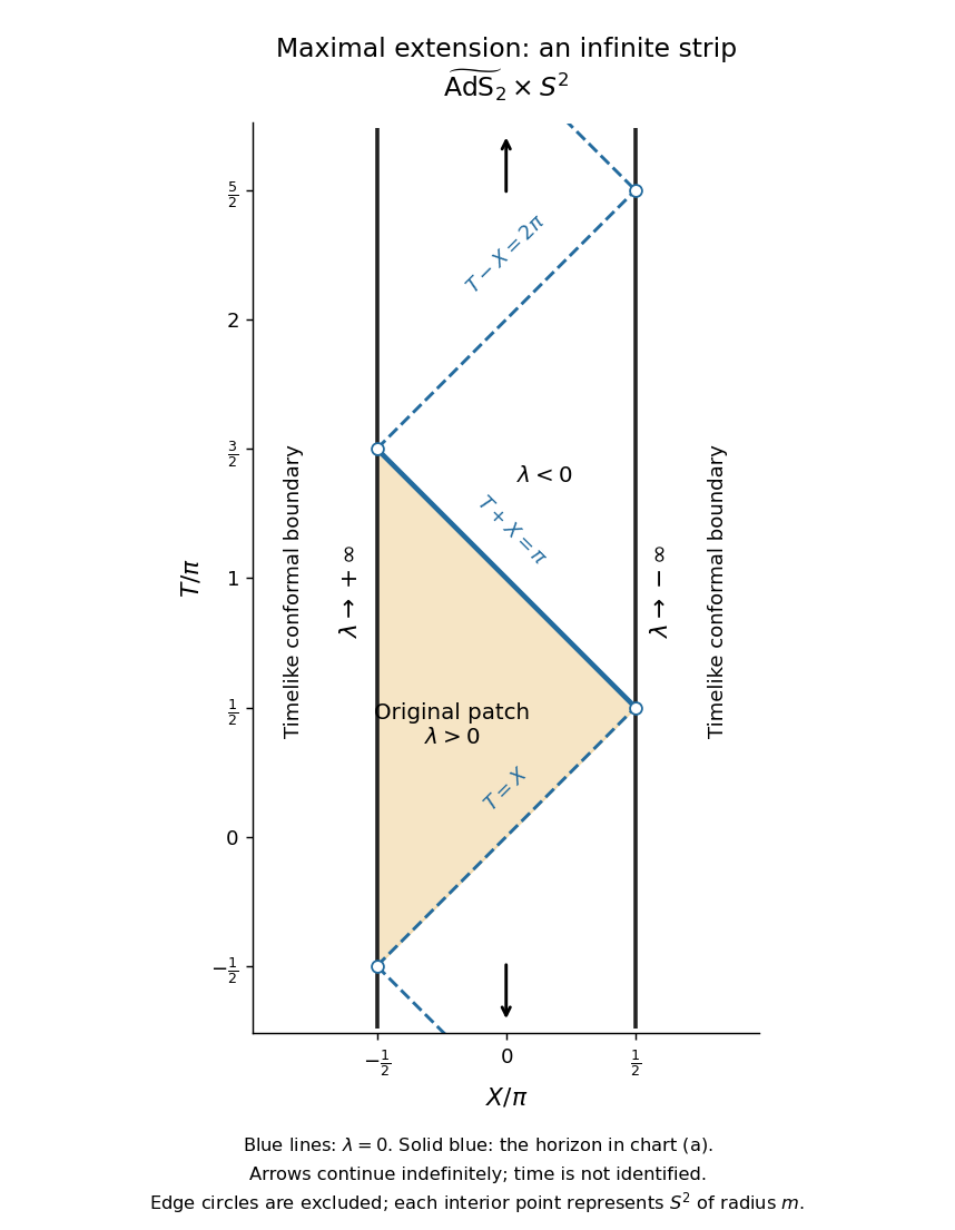
Penrose diagram of the maximal Bertotti-Robinson spacetime extension, with the original patch and all zero-level Killing horizons
. Details. 
Finally, these timelike edges are conformal boundaries, not omitted regular points of a further spacetime extension. One way to establish maximality is geodesic completeness. The two-dimensional anti-de Sitter spacetime factor embeds locally as in a flat space with metric signature . Along an affinely parametrized geodesic with constant , the ambient equation isIts oscillatory, linear or hyperbolic solutions for negative, zero or positive exist for all real affine parameters and lift to the universal cover. The two-sphere is also geodesically complete, and geodesics of the product split into geodesics of its factors. Hence is geodesically complete. A proper regular spacetime extension would furnish a geodesic reaching its boundary in finite affine parameter, contradicting that completeness. This proves that the displayed simply connected analytic spacetime is maximal.
Articles by others on the same topic
There are currently no matching articles.