Past exam of the mathematical and Computational Biology course of the University of Cambridge / 2024 / Paper 2 / A3

The first instruction asks for maximization, whereas the later parts refer to minimization. For the literal maximization task, minimize the negative objective:

import numpy as np
from scipy import optimize as opt


def f(x):
    return 1 + np.exp(-x*x/5) * np.sin(5*x)


maximum = opt.minimize(lambda z: -f(z[0]), x0=[-1.0])
print(maximum.x[0], f(maximum.x[0]))

This gives a local maximum near $x = - 0.927662$ , $f (x) = 1.839576$ . If minimization was intended, use opt.minimize(lambda z: f(z[0]), x0=[-1.0]), which instead returns a local minimum near $x = - 1.546182$ , $f (x) = 0.384751$ . The optimizer's stopping criterion establishes local numerical convergence, not a certificate of a global optimum.

b

 0  0

Solution

 0  0

Plot the entire stated interval:

import matplotlib.pyplot as plt

x_grid = np.linspace(-4, 4, 1500)
plt.plot(x_grid, f(x_grid))
plt.xlabel("x")
plt.ylabel("f(x)")
plt.show()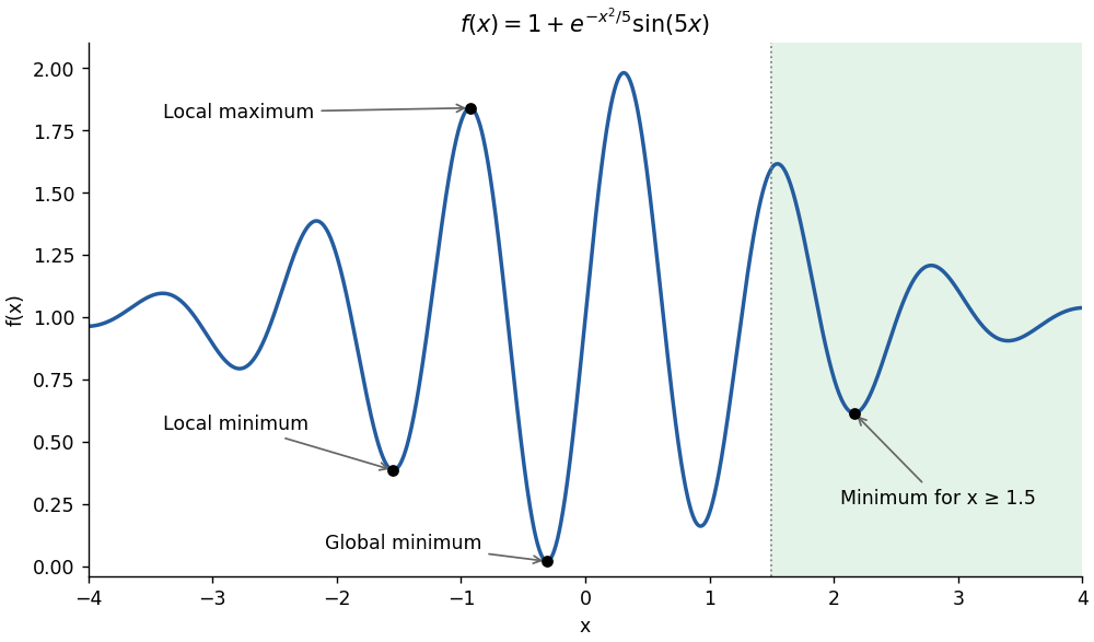

The oscillating objective has several wells. A local search starting at

- 1

need not reach the deepest one, which is near

- 0.309

. For the literal maximization in part (a), no minimum was being sought at all. Under the intended minimization interpretation, the result near

- 1.546

belongs to a different attraction region from the global minimum.

Figure 1.
Local extrema, the global minimum and the constrained minimum of the oscillatory objective
. **Details**.

c

 0  0

Solution

 0  0

Use reproducible random starts and retain the best successful result:

rng = np.random.default_rng(2024)
starts = rng.uniform(-4, 4, size=100)
results = [opt.minimize(lambda z: f(z[0]), x0=[x0]) for x0 in starts]
successful = [result for result in results if result.success]
best = min(successful, key=lambda result: result.fun)
print(best.x[0], best.fun)

The estimate is $x_{m i n} ≃ - 0.309213$ , $f_{m i n} ≃ 0.0192409$ . This random-restart optimization improves coverage of the different attraction regions, but their number alone does not guarantee global optimality.

Here an analytic check is possible. For

∣ x ∣ \geq π /5

, the envelope gives

f (x) \geq 1 - e^{- π^{2} /125} ≃ 0.0759

, above the candidate. On

[0, π /5]

f \geq 1

. In the remaining interval

[- π /5, 0]

, the derivative condition is equivalent, with

z = - x

, to

cot (5 z) = 0.08 z

. The left side decreases strictly from

+ \infty

- \infty

while the right side increases, giving one minimum. This certifies the selected well as global rather than relying only on the restart experiment.

d

 0  0

Solution

 0  0

Set

x = 1.5 + e^{y}

. Every finite unconstrained value of

y

then gives an allowed point with

x > 1.5

def transformed(y):
    return f(1.5 + np.exp(y[0]))


result = opt.minimize(transformed, x0=[0.0])
x_interior = 1.5 + np.exp(result.x[0])
x_best = min([1.5, x_interior], key=f)
print(x_best, f(x_best))

Explicitly checking

x = 1.5

covers the boundary omitted by the exponential transformation. The minimum is $x ≃ 2.164817$ , $f (x) ≃ 0.614056$ , whereas

f (1.5) ≃ 1.59810

Constraint reparameterization enforces feasibility but does not remove nonconvexity. In this example,

f \geq 1

up to the next negative-sine lobe, the derivative has one minimum in that lobe, and for

x \geq 4 π /5

the envelope gives

f (x) \geq 1 - e^{- 16 π^{2} /125} ≃ 0.7173

. Thus later oscillations cannot improve on the displayed constrained minimum.

Past exam of the mathematical and Computational Biology course of the University of Cambridge / 2024 / Paper 2 / A3

a

Solution

b

Solution

c

Solution

d

Solution

 Ancestors (11)

 Discussion (0)

 Articles by others on the same topic (0)

Past exam of the mathematical and Computational Biology course of the University of Cambridge / 2024 / Paper 2 / A3

 Discussion (0)  Subscribe (1)

 Discussion (0)