The S-Plus input and the data table differ in one entry: the former uses for the first year in the second male age group, whereas the table has . The displayed coefficients are reproduced by the software vector with , so that is the input analysed here. Using instead would give a different fit, including an intercept of rather than .
The factor grid has rows. Its first factor varies fastest, so the five years run within each age group, and the age groups run within each sex. All three predictors are regression factors: in particular the year coefficients are category contrasts, not a fitted linear slope in calendar time. Under reference-level coding, take the first year, youngest age group and men as the reference levels in a regression factor. Write for women and for men, and for the other year and age indicators. The normal linear model isThe star in the formula includes both main effects and their statistical interaction. There are twelve coefficients: an intercept, four year contrasts, one sex contrast, three age contrasts and three sex-by-age contrasts. Year effects are assumed common across all sex-age combinations; there is no year interaction term. Independent errors with common variance are additional assumptions of the reported exact tests.
The least-squares estimator is , where has rank twelve. Under the normal linear model,and these quantities are independent. This standard normal-projection theorem gives and estimated coefficient standard errors . A coefficient estimate divided by its standard error has a Student t-distribution with 28 degrees of freedom under its zero-coefficient null. These are the printed t statistics and two-sided p-values; a printed zero is rounding, not a probability of exactly zero. The option suppresses the coefficient-correlation display.
The fitted intercept is the expected percentage for the reference sex, age and year. Relative to that year, the year changes are percentage points. The last two are individually significant at the conventional five-percent level; the first two are not. The sex coefficient is the female-minus-male difference in the youngest group. The male age changes are points. Adding the three interaction term coefficients gives the female age changes . Thus the sex gap shrinks with age. An individual insignificant interaction term coefficient does not justify deleting the whole interaction: the joint partial F-test for the three interaction terms gives on degrees of freedom, with .
The regression residuals are observed minus fitted percentages; their printed five-number summary describes their spread. Direct calculation gives , so the residual standard error isThe coefficient of determination is . The overall F-test compares all eleven non-intercept coefficients with zero:Under the null it has an F-distribution on degrees of freedom; its very small p-value shows substantial explained variation. This does not independently validate the Gaussian error assumptions. Survey percentages can have different sampling variances and correlations, and the survey denominators and design are not supplied. The output's exact inferential interpretation is conditional on the stated normal linear model.
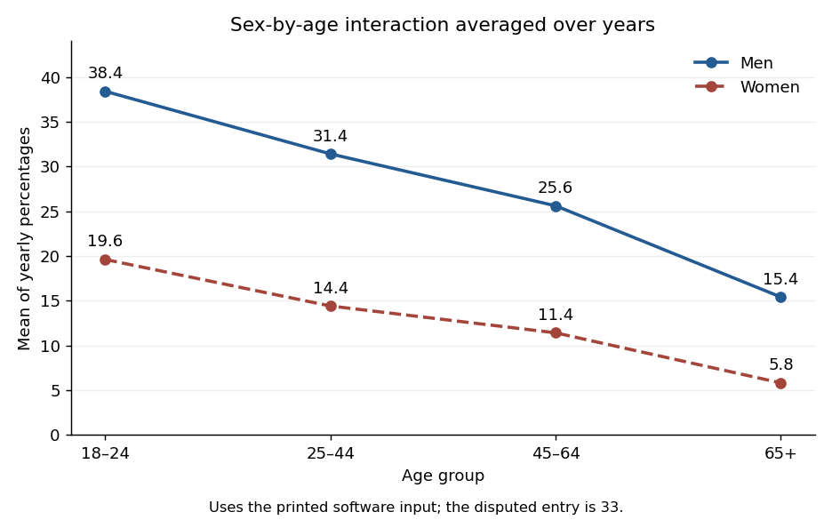
The final command makes an interaction plot, not another regression fit. Its points are arithmetic averages over the five years for each sex-age combination. It draws two decreasing, nonparallel lines, with coordinatesTheir gaps are percentage points, illustrating the sex-by-age statistical interaction. The average uses the software vector's disputed entry, consistently with the displayed fit. These are means of percentages, not denominator-weighted pooled prevalence estimates.

Articles by others on the same topic
There are currently no matching articles.