Past exam of the mathematics course of the University of Cambridge / 2003 / iii / Paper 38 (Applied Statistics)

The S-Plus input and the data table differ in one entry: the former uses $33$ for the first year in the second male age group, whereas the table has $22$. The displayed coefficients are reproduced by the software vector with $33$, so that is the input analysed here. Using $22$ instead would give a different fit, including an intercept of $36.175$ rather than $37.275$.

The factor grid has $5\times 4\times 2=40$ rows. Its first factor varies fastest, so the five years run within each age group, and the age groups run within each sex. All three predictors are regression factors: in particular the year coefficients are category contrasts, not a fitted linear slope in calendar time. Under reference-level coding, take the first year, youngest age group and men as the reference levels in a regression factor. Write $s=1$ for women and $0$ for men, and $I_{yk},I_{aj}$ for the other year and age indicators. The normal linear model isThe star in the formula includes both main effects and their statistical interaction. There are twelve coefficients: an intercept, four year contrasts, one sex contrast, three age contrasts and three sex-by-age contrasts. Year effects are assumed common across all sex-age combinations; there is no year interaction term. Independent errors with common variance are additional assumptions of the reported exact tests.

The least-squares estimator is $\hat{b}=(X^{T}X{)}^{-1}{X}^{T}P$, where $X$ has rank twelve. Under the normal linear model,and these quantities are independent. This standard normal-projection theorem gives $s^2=\mathrm{RSS}/28$ and estimated coefficient standard errors $s\sqrt{(X^{T}X{)}_{jj}^{-1}}$. A coefficient estimate divided by its standard error has a Student t-distribution with 28 degrees of freedom under its zero-coefficient null. These are the printed t statistics and two-sided p-values; a printed zero is rounding, not a probability of exactly zero. The option suppresses the coefficient-correlation display.

The fitted intercept $37.275$ is the expected percentage for the reference sex, age and year. Relative to that year, the year changes are $0.375,0.500,1.750,3.000$ percentage points. The last two are individually significant at the conventional five-percent level; the first two are not. The sex coefficient $-18.8$ is the female-minus-male difference in the youngest group. The male age changes are $-7,-12.8,-23$ points. Adding the three interaction term coefficients gives the female age changes $-5.2,-8.2,-13.8$. Thus the sex gap shrinks with age. An individual insignificant interaction term coefficient does not justify deleting the whole interaction: the joint partial F-test for the three interaction terms gives $F=18.6822$ on $(3,28)$ degrees of freedom, with $p\simeq 7.46\times 10^{-7}$.

The regression residuals are observed minus fitted percentages; their printed five-number summary describes their spread. Direct calculation gives $\mathrm{RSS}=60.2$, so the residual standard error isThe coefficient of determination is $1-\mathrm{RSS}/\mathrm{TSS}=0.985827$. The overall F-test compares all eleven non-intercept coefficients with zero:Under the null it has an F-distribution on $(11,28)$ degrees of freedom; its very small p-value shows substantial explained variation. This does not independently validate the Gaussian error assumptions. Survey percentages can have different sampling variances and correlations, and the survey denominators and design are not supplied. The output's exact inferential interpretation is conditional on the stated normal linear model.

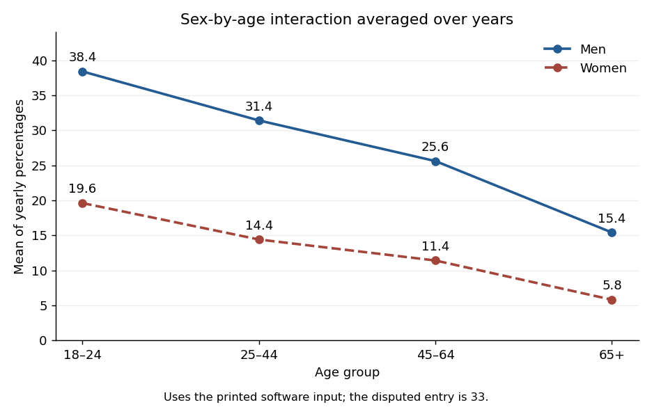
The final command makes an interaction plot, not another regression fit. Its points are arithmetic averages over the five years for each sex-age combination. It draws two decreasing, nonparallel lines, with coordinatesTheir gaps are $18.8,17.0,14.2,9.6$ percentage points, illustrating the sex-by-age statistical interaction. The average uses the software vector's disputed entry, consistently with the displayed fit. These are means of percentages, not denominator-weighted pooled prevalence estimates.

The prose names a second year that differs from the table label. The calculations use the four supplied counts, interpreting the first and second rows as the two displayed periods; no numerical conclusion depends on resolving that label discrepancy.

The first generalized linear model treats the four counts as independent Poisson random variables, with a log link and both row and column regression factors. The row-by-column interaction makes the log-linear model saturated. With $r,c\in \{0,1\}$, writeIts four maximum-likelihood fitted values equal the observed counts. Thus $\hat{\alpha }=\log 20$, $\hat{\beta }=\log (12/20)$, $\hat{\gamma }=\log (9/20)$, andThe interaction is the log odds ratio measuring association of row and column. Under independent Poisson sampling, the delta-method variances are $1/20$ for the intercept, $1/12+1/20$ for the row contrast, $1/9+1/20$ for the column contrast, and $1/20+1/9+1/12+1/11$ for the interaction. Their square roots reproduce the printed standard errors. Although the software labels the standardized ratios as t values, these are asymptotic normal Wald statistics, with known Poisson dispersion one, not exact finite-df Student tests.

The statistical saturated model has zero residual deviance and zero residual degrees of freedom; this is a perfect interpolation, not evidence of predictive adequacy. The null deviance $5.016056$ compares the four observed counts with an intercept-only model, whose four fitted means are $52/4=13$. Fisher scoring is the numerical score/information iteration used to fit the model; the iteration count is a convergence report, not a test statistic.

Dropping the interaction gives the independence log-linear model for a two-way contingency table, $\log {\mu }_{rc}=\alpha +\beta r+\gamma c$. Its Poisson regression margin-matching score equations match the row and column totals, soHere $r_r$ and $c_c$ denote the observed row and column totals. In particular the fitted row multiplier is $23/29$, the column multiplier is $20/32$, and the intercept is $\log (29\cdot 32/52)=2.881788$. These produce the second coefficient table. Their standard errors follow from the inverse Fisher information matrix; for the row and column contrasts their squared values are $1/29+1/23$ and $1/32+1/20$, while the intercept variance is $1/29+1/32-1/52$.

The Poisson deviance relative to the saturated fit isThe linear terms cancel because fitted and observed totals agree. The additive model has three coefficients, leaving one degree of freedom. Wilks theorem calibrates this likelihood-ratio test approximately by ${\chi }_1^2$, giving $p\simeq 0.2164$. The interaction Wald test instead gives $p\simeq 0.2192$; the two are only asymptotically equivalent.

Fisher's exact test conditions on both margins under independence. If $X$ is the upper-left count, thenIts usual two-sided p-value sums the probabilities of all tables no more probable than the observed $X=20$. That sum is $0.259724$, reproducing the output without an asymptotic approximation. It tests the same absence of row-column association, but conditioning and discreteness explain the numerical difference from the likelihood-ratio test.

In ordinary language, the male proportion among the cases is $20/29\simeq 69.0\%$ in the first row and $12/23\simeq 52.2\%$ in the second. The estimated case-sex odds ratio is $2.037$, but its approximate 95-percent confidence interval is wide, $(0.655,6.338)$. These small samples do not give convincing evidence that the sex composition of cases changed between the two periods. Failure to reject is not evidence that the compositions are exactly equal. Nor do these counts establish a male-to-female disease-incidence ratio or an incidence trend: population denominators and comparable ascertainment would be needed for those interpretations.

For independent Bernoulli random variables, the log-likelihood isEvery likelihood factor is at most one, so $\ell \le 0$. In the statistical saturated model, choose ${\hat{\pi }}_i=y_i$ independently for each observation. The probability of each realised response is then exactly one. With the continuous convention $0\log 0=0$, the Bernoulli saturated log-likelihood is thereforeThe inclusion of probabilities zero and one is important: if the parameter space required $0<{\pi }_i<1$, zero would be the supremum approached at the boundary, rather than an attained maximum.

The first fit is a Bernoulli logistic-regression model for the probability of a positive response. Its fitted linear predictor isand its fitted probability is $\hat{\pi }=(1+e^{-\hat{\eta }}{)}^{-1}$. There are eight coefficients. The null degrees of freedom identify $n=200$, and the residual degrees of freedom are $200-8=192$.

Each slope is a change in the log odds per unit of its covariate, holding the others fixed. Exponentiating gives conditional odds ratios; for example a ten-unit glucose increase multiplies fitted odds by $e^{10(0.032115958)}=1.379$, and a ten-year age increase by $e^{10(0.041182353)}=1.510$. These are changes in odds, not multiplicative changes in probability, and the observational associations are not automatically causal effects. The intercept corresponds to all numerical covariates being zero, generally an extrapolation beyond meaningful subjects.

The standard errors come from the inverse Fisher information matrix of the logistic regression. With binomial dispersion parameter fixed at one, the displayed t ratios are asymptotic normal Wald statistics. In the full fit, glucose and the pedigree measure have clear individual evidence of nonzero slopes, with two-sided $p\simeq 2.09\times 10^{-6}$ and $0.00609$. The body-mass and age terms are borderline, with $p\simeq 0.0504$ and $0.0618$; pregnancy count is weaker, $p\simeq 0.110$. Blood pressure and skinfold have little individual evidence after adjustment. These labels should not be converted into a claim that the weaker predictors have no effect, or used as automatic model-selection rules.

A deviance residual here isIts square is the observation's contribution to binomial deviance, so the squared residuals sum to the printed residual deviance. The five-number summaries describe the distribution of these signed residuals. The null deviance $256.4142$ belongs to an intercept-only logistic regression; the full fitted deviance is $178.3907$. Four Fisher scoring iterations record convergence of the numerical likelihood fit.

The second model uses only glucose:Its two coefficients leave $198$ residual degrees of freedom. A ten-unit glucose increase multiplies its fitted odds by $e^{0.3778371}\simeq 1.459$. This differs from the adjusted multiplier $1.379$, because the models condition on different covariates; both adjustment and noncollapsibility of the odds ratio can change logistic coefficients. The glucose-only model has deviance $207.3727$, so its maximized log-likelihood is lower than the full model's.

For these fixed-dimensional nested models, analysis of deviance and Wilks theorem giveThus the additional six predictors collectively improve the glucose-only model, even though several individual Wald tests are not significant. These comparisons assume independent subjects, an appropriate logistic mean structure, full rank, and regular finite parameter estimates without separation.

It would be incorrect to infer that absolute fit is good merely because $178.39<192$. Individual Bernoulli deviance need not have a chi-squared calibration: there is just one binary observation per saturated probability, and the saturated dimension increases with sample size. A simple counterexample is an intercept-only model with true probability $1/2$, for which $D/n\to 2\log 2$, not one. For absolute adequacy, inspect residual patterns and predicted-risk calibration, use meaningful grouped comparisons when appropriate, or calibrate a chosen fit statistic by parametric bootstrap. The regular nested-model tests above are not subject to that saturated-model dimensionality problem. Only the displayed summaries and a few example rows are supplied, so patient-level diagnostics or complete numerical refitting cannot be reconstructed from this page alone.

Use $\alpha$ for the intercept, to avoid confusing it with the observation means. Let $e_i=\exp (\hat{\alpha }+{\hat{\beta }}^T{x}_i)$ be the fitted Poisson regression mean. Apart from constants, its log-likelihood isAt a finite interior maximum-likelihood estimate, the intercept score equation gives the Poisson regression margin-matching score equations:The statistical saturated model fits each mean to $y_i$, taking the boundary mean zero if $y_i=0$. Subtracting fitted from saturated log-likelihood gives the Poisson devianceThe intercept balance cancels the sum of linear terms. ConsequentlyThe unsimplified formula makes nonnegativity transparent; individual terms in the simplified formula need not each be positive.

For the deviance goodness-of-fit test, if the fitted design has rank $r$, compare a suitably calibrated $D$ with ${\chi }_{n-r}^2$, rejecting for large values. This approximation applies in a regular large-count regime, such as a fixed set of cells with increasing exposure and positive fitted proportions. It is not automatically accurate for many sparse Poisson observations. Check residual patterns and overdispersion; where the approximation is doubtful, simulate independent Poisson random variables with fitted means, refit each sample, and use a parametric bootstrap distribution of the same statistic. A large p-value means no detected lack of fit, not proof of the model. If a finite interior estimate fails to exist, the score proof needs a boundary-limit interpretation; for example all-zero data give a supremum with every fitted mean tending to zero and limiting deviance zero.

Here the negative binomial distribution has mean parameter $\mu >0$ and size parameter $\theta >0$. Its support in the original PDF is all nonnegative integers; a finite endpoint appearing in the TeX aid would be incorrect. The probability generating function, obtained from the generalized binomial series, isDifferentiating at one gives $G^{\prime }(1)=\mu$ and $G^{\prime \prime }(1)={\mu }^2(1+1/\theta )$. Since the variance is $G^{\prime \prime }(1)+G^{\prime }(1)-G^{\prime }(1{)}^2$, this provesThe extra positive term explains its overdispersion relative to a Poisson distribution.

For one observation, write the log-likelihood asThe mean score function and its cross derivative areTaking expectations gives $I_{\mu \theta }=-\mathbb{E}({\partial }_{\theta }{u}_{\mu })=0$. In addition,For reference, with $\psi$ the digamma function, the size score function isIts variance $I_{\theta \theta }$ is finite and positive for finite positive $\mu ,\theta$. Thus negative binomial mean-size parameter orthogonality makes the expected Fisher information matrix diagonal. For an independent identically distributed sample and a regular identifiable interior true parameter, asymptotic normality of a maximum likelihood estimator givesHence the asymptotic correlation is zero. This is first-order asymptotic independence, not a claim of exact finite-sample independence. Indeed the mean score yields $\hat{\mu }=\bar{y}$ at an interior fit, while the size fit also depends on the observed dispersion. The argument excludes a true boundary such as the Poisson limit $\theta =\infty$.

The independence analysis is not justified without further assumptions. Three binary responses from the same subject generally remain correlated after conditioning on baseline covariates and treatment. The fitted independent-Bernoulli likelihood discards that correlation and gives incorrect model-based standard errors and tests if it is present. Positive within-subject correlation commonly makes those errors too small.

There is an important distinction between estimating the mean and estimating uncertainty. If the stated marginal logistic regression is correct and responses are fully observed, the independence score ${\sum }_{i,j}{w}_{ij}(Y_{ij}-m_{ij})$ still has zero expectation. With independent subjects and regularity, its root can consistently estimate marginal coefficients despite within-subject dependence; a subject-level sandwich covariance matrix is then needed. True independence is a special case in which the original standard errors would be appropriate.

Dropout creates a separate issue. Restricting that score to observed responses need not preserve its zero expectation if observation depends on the response history or unseen depression outcomes. Therefore both point estimates and uncertainty may be wrong. Neither random treatment assignment nor baseline adjustment alone establishes an ignorable missingness mechanism. We need a model matched to the scientific estimand and explicit assumptions about missing data.

For a population question use a population-averaged logistic model for repeated binary outcomes. Code $z_i=1$ for the new treatment and $0$ for the control, with visit times $t_j=2j$ months for $j=1,2,3$. Let $w_{ij}=(1,z_i,x_i^T,t_j{)}^T$, ${\gamma }_M=({\alpha }_M,{\varphi }_M,{\beta }_M^T,{\delta }_M{)}^T$, andDifferent subjects are independent. Each response has a Bernoulli distribution with this marginal mean, but no independence of a subject's three responses is assumed. The linear time effect and absence of treatment-by-time interaction are substantive mean assumptions; if inappropriate they can be replaced by time indicators and interaction terms.

For complete data, set $m_i=(m_{i1},m_{i2},m_{i3}{)}^T$, $A_i=\mathrm{diag}(m_{ij}(1-m_{ij}))$, and $D_i=\partial m_i/\partial {\gamma }_M^T=A_i{W}_i$, where $W_i$ has rows $w_{ij}^T$. A working exchangeable correlation matrix has unit diagonal and off-diagonal value $\rho \in (-1/2,1)$; set $V_i=A_i^{1/2}C(\rho )A_i^{1/2}$. The generalized estimating equation isWith correct means and independent subjects, a positive-definite working covariance matrix and regularity give consistency even if the working correlation is wrong. Write $H={\sum }_i{D}_i^T{V}_i^{-1}{D}_i$ and $u_i=D_i^T{V}_i^{-1}(Y_i-m_i)$. The fitted subject-level sandwich covariance matrix isevaluated at the estimates. This inference is asymptotic in the number of independent subjects, not the number of visits.

For the actual incomplete data, define $R_{ij}=1$ if visit $j$ is observed, with $R_{i0}=1$ and monotone dropout. Let ${\mathcal{H}}_{i,j-1}$ contain treatment, baseline covariates and responses observed before visit $j$. Under sequential missing at random, specifyThe assumption is that the retention decision, conditional on this history, does not additionally depend on unseen current or future outcomes. Fit the $q_{ij}$, for example by visit-specific logistic regressions. A simple valid choice uses working independence and the inverse-observation-weighted estimating equations for longitudinal dropout:Terms with $R_{ij}=0$ are zero and require no missing response. Given the full response vector, sequential missing at random makes $\mathbb{E}(R_{ij}/{\rho }_{ij}\mid Y_i,z_i,x_i)=1$. Consequently the weighted score has the same expectation as the complete-data score, proving its mean-zero property. Correct retention probabilities, positivity and a correctly specified marginal mean are required. Use cluster-robust uncertainty, accounting for fitted retention-model coefficients, or resample entire subjects and refit both models. Under missing completely at random, the simpler unweighted observed-response GEE can suffice; ordinary unweighted GEE is not valid under arbitrary history-dependent missing at random.

The treatment coefficient gives a population conditional-on-baseline odds ratio $e^{{\varphi }_M}$ at each visit. To communicate an absolute population treatment benefit, standardize predicted probabilities over the full baseline population, rather than only completers:A causal reading additionally uses the randomized controlled trial assignment, consistency of the treatment definition, no interference and the dropout assumptions; the statistical model alone does not supply those conditions.

For conditional individual response profiles use a logistic random-intercept model for repeated binary outcomes. Introduce a subject effect $B_i\sim N(0,{\tau }^2)$ independently across subjects and independently of treatment and baseline covariates, under the specified model. Conditional on $B_i,z_i,x_i$, assume the three responses are independent Bernoulli random variables withHere $B_i$ is persistent unmeasured subject heterogeneity and ${\tau }^2$ its variance. It induces dependence after integration: for distinct visits, the response covariance is ${\mathrm{Cov}}_B(p_{ij}(B),p_{ik}(B))$, generally positive. This is a complete joint generalized linear mixed model, unlike a mean-only GEE specification.

Under missing at random conditional on the observed responses and baseline variables, with distinct parameters for missingness and outcomes, the missingness model is ignorable for likelihood inference. Let ${\mathcal{O}}_i=\{j:R_{ij}=1\}$. The outcome observed-data likelihood isThe omitted Bernoulli factors sum to one over missing outcomes. Fit the fixed coefficients and ${\tau }^2$ by maximizing this integrated likelihood, with suitable quadrature or another justified integration method. If $\tau =0$, use the limiting point-mass model. Correct response and random-effect distributions, identifiable coefficients and regularity are needed; the latent distribution assumption is not merely a convenient working covariance.

For patient $i$, combine the fitted model with the posterior density of $B_i$ proportional to its normal density times that patient's observed Bernoulli factors. Integrating $p_{ij}(b)$ over this posterior gives a patient-specific predicted response profile. The treatment odds ratio for a fixed $b$ and the same baseline variables is $e^{{\varphi }_C}$. This conditional contrast does not by itself identify each person's unobserved causal treatment effect: a parallel-arm trial observes only one treatment per person. Random slopes or heterogeneous treatment effects require further modelling and sufficient information; they are not implied by fitting a random intercept.

The population-averaged logistic regression describes $P(Y_{ij}=1\mid z_i,x_i)$ after averaging over unmeasured individual heterogeneity. Its intercept is a marginal log odds at reference baseline values and time zero, its treatment coefficient is a population conditional-on-baseline log odds ratio, and its time coefficient is the change in that marginal log odds per month. Time zero is an extrapolation here because the recorded visits begin later; centring time at the first visit would give a more interpretable intercept.

In the random-intercept logistic model, the intercept is instead the conditional log odds for a subject with $B_i=0$. The treatment and time coefficients apply at fixed $B_i$; the subject's actual intercept is ${\alpha }_C+B_i$. Even with a treatment-independent random intercept, the conditional and marginal coefficients generally differ through noncollapsibility of the odds ratio. Indeed, if $\eta ={\alpha }_C+{\varphi }_{C}z+{\beta }_C^{T}x+{\delta }_{C}t$, marginalization giveswhich is not generally a logistic curve with the same linear coefficients. To quantify random-intercept attenuation of marginal logistic slopes, let $p_B={\mathrm{logit}}^{-1}(\eta +B)$. ThenFor a nondegenerate finite random intercept this derivative lies strictly between zero and one and usually varies with $\eta$. Thus the marginal treatment contrast is an integrated, attenuated version of the conditional contrast, and the marginal time slope need not be constant. One should not equate the two sets of coefficients, even in a randomized controlled trial without treatment confounding.

For missing completely at random, an unweighted observed-response GEE with cluster-robust standard errors can consistently fit the marginal mean, and a correctly specified integrated GLMM likelihood is valid as well. Under missing at random depending on previous observed outcomes, ordinary unweighted GEE is generally biased because the remaining responses are selected by informative observed history. Correct inverse-observation-weighted estimating equations for longitudinal dropout recover the marginal target under the sequential MAR and positivity assumptions already stated. Covariate-only observation mechanisms are a simpler special case in which correctly conditioned unweighted mean equations can remain valid.

A correctly specified joint response GLMM, fitted by observed-data likelihood, is valid under ignorable missing at random with distinct parameters, including dependence of missingness on observed response history. This is a likelihood property, not a claim that every mixed model automatically fixes missingness. Under missing not at random, neither ordinary GEE, MAR-based weights nor a response-only GLMM is generally valid; the unseen-outcome dependence requires further modelling and sensitivity assumptions.

First investigate what predicts dropout among variables actually observed, record reasons where possible, and seek additional outcome follow-up. Dependence on observed history alone can be missing at random; informative dependence on unseen responses or latent heterogeneity requires a missing not at random analysis. Observed data do not ordinarily distinguish MAR from all MNAR explanations.

An explicit selection model for informative longitudinal dropout can augment a joint response model $f_{\vartheta }(Y_i\mid z_i,x_i)$ by dropout hazards. Define $R_{ij}$ as above and, among subjects retained through visit $j-1$, putOmit the previous-response term at the first visit. A nonzero $\kappa$ makes dropout depend on the currently missing response. For monotone observation indicators $r_i$, letThe appropriate observed-data likelihood isThus a patient's dropout pattern contributes information in the model; dropping the $g_{\eta }$ factor is not justified under this informative mechanism.

Another option is a shared-parameter model for informative dropout: retain the conditional Bernoulli response model, but let the dropout logit contain the same latent effect, for example $a_j+c^T{x}_i+d{z}_i+\lambda Y_{i,j-1}+{\kappa }_B{B}_i$. Conditional on the shared effect and observed history the processes can be independent, while marginally dropout remains associated with unseen responses. The joint likelihood must integrate the response factors and dropout factors together over $B_i$. A response-only mixed-model fit does not generally account for this dependence.

Because $\kappa$ or ${\kappa }_B$ can be weakly identified from the observed outcomes, report sensitivity of the treatment conclusion to plausible informative-dropout assumptions. One can fix a range of these dependence parameters and refit, or use pattern-mixture sensitivity analysis that shifts the imputed post-dropout log odds by a specified amount from the MAR prediction. Present population risks and treatment contrasts across these scenarios with their uncertainty. These are explicit identifying assumptions, not an empirical test proving which missingness mechanism is true. Neither a complete-case analysis nor carrying forward the last response supplies such a justification.