In a coordinate chart the Lie derivative of a function and Lie derivative of a vector field areThe Lie derivative of a tensor field is the extension that respects tensor products and contractions. For a covector field , differentiate the scalar pairing to obtain . In components this givesThus for a mixed rank-two tensor field, the coordinate tensor Lie derivative isEach upper index contributes a negative derivative of the generator and each lower index a positive one. Explicitly, for type ,These rules follow by expanding in coordinate vector and covector bases and using the product rule; they define the extension independently of that basis. For a symmetric connection, replacing the partial derivatives by covariant derivatives leaves these expressions unchanged because the connection terms cancel.
For the commutator identity, on functions. On a vector field , the Jacobi identity gives . The difference is a tensor derivation respecting contractions. Since it vanishes on functions and vectors, pairing a covector with every vector shows it vanishes on covectors. Product expansions then show it vanishes on every tensor. This proves the commutator identity for Lie derivatives:A Killing vector generates infinitesimal isometries, meaning , equivalently the Killing equation for the metric Levi-Civita connection. Linearity in the generator gives for real constants whenever are Killing. The identity above likewise gives . Thus the Killing fields form a real Lie algebra; arbitrary nonconstant coefficients would introduce additional derivative terms.
For the rotating star, the hypothesis that there are exactly two independent Killing fields means with constant coefficients. Axial symmetry supplies a periodic rotation flow; with the stated asymptotic normalization its generator is and its period is . Pullback by this flow acts on the Killing algebra, so . In the basis , has matrixIts real eigenvalues are and zero, so the exponential identity forces . The remaining matrix squares to zero; its exponential is then , forcing . The two-dimensional Killing algebra with a periodic generator is abelian result therefore gives .
This uses genuine periodic axial symmetry and the two-dimensional Killing algebra. Mere limits of vector components do not by themselves justify differentiating those limits to evaluate their bracket; the periodic-flow argument avoids that gap. With the usual differentiable asymptotically flat falloff one can also take the bracket at infinity and use independence of the limiting time and angular generators to set both constants to zero.
Work to first order in a metric perturbation , with , raising perturbation indices with and discarding quadratic terms. The Christoffel symbols areUsing the printed curvature convention gives the linearized Riemann curvature operatorFor definiteness contract . The corresponding first-order Ricci tensor isThis is the reversed sign convention specified in curvature-sign convention in Killing derivative identities; the vacuum equation is unaffected by an overall curvature sign.
An infinitesimal passive coordinate change changes the perturbation by . Substitution into gives zero change, since partial derivatives commute. Equivalently the change in curvature is the Lie derivative of the background curvature, which vanishes in Minkowski spacetime. Thus linearized curvature, and the linearized Weyl tensor in vacuum, are gauge-invariant tidal observables, whereas individual components of are generally gauge dependent.
The trace-reversed metric perturbation transforms by . Its divergence changes by . Solving therefore imposes Lorenz gauge in linearized gravity, . With the stated sign convention the Einstein tensor isso the linearized vacuum field equation becomes . The residual gauge symmetry of linearized gravity has . This makes a hyperbolic evolution problem after the gauge condition and its initial consistency constraints have been imposed.
To separate actual gauge invariants from a gauge choice, use gauge-invariant Minkowski perturbations. For spatial indices contracted with , decomposewhere , and . Spatial falloff or Fourier-mode conventions fix the decomposition. Write and with . Direct substitution in the gauge change givesHence the invariant combinations areA representative with has , and . The explicit vacuum constraints for gauge-invariant Minkowski perturbations follow fromFor a nonzero spatial Fourier mode, or regular decaying fields on all space, forces , then forces , and the spatial trace gives , hence . Only remains. This removal of the scalar and vector sectors does not exclude singular Coulomb perturbations outside a source, boundary-driven harmonic potentials or spatially homogeneous modes; those require separate boundary and gauge conventions.
For a propagating plane mode , the wave equation gives . A transverse-traceless spatial tensor perpendicular to a fixed propagation direction has two independent components. For propagation along , define the physical strain in this mostly-minus convention, so the spatial line element is . It has the formThese are the two gravitational wave polarizations, plus polarization and cross polarization. A rotation in the transverse plane rotates the polarization pair through twice the angle; cross is plus rotated through degrees. Lorenz constraints and residual gauge freedom give the same count: ten symmetric metric components minus four constraints and four gauge freedoms leave two radiative degrees of freedom.
In transverse-traceless gauge, particles initially at rest keep fixed spatial coordinates since , but their measured separation changes. For a short separation of length in unit direction , . The gauge-invariant curvature gives the corresponding geodesic deviation:Here the last equation is in a freely falling orthonormal frame, with the printed reversed curvature convention. Coordinate separation and physical separation must not be confused. The linearized vacuum equations describe propagation and tidal measurements; wave energy transfer and an effective wave stress-energy tensor arise at quadratic order, beyond the linear approximation.
Use the metric Levi-Civita connection and hold the covariant potential fixed when varying the metric. Symmetry of the connection cancels its terms in the electromagnetic field tensor:The Electromagnetic Bianchi identity follows from commuting partial derivatives, or and . Written covariantly it is , since total antisymmetrization also cancels the symmetric connection terms. Hence without using any field equation.
For the potential variation, . Antisymmetry in the Maxwell action giveswhere the second equality is integration by parts followed by relabeling; compactly supported variations, or vanishing boundary variations, remove the surface term. Arbitrary therefore give the source-free Maxwell equationsNo gauge fixing of is needed for this variational calculation.
In signature define the Hilbert stress-energy tensor by . Since the independent covariant potential makes metric independent,Combining these two terms yields the electromagnetic stress-energy tensorEquivalently . The overall stress-variation sign has been matched to the signature and action. As a check, in an orthonormal frame and for a nonzero field; copying a mostly-plus formula without changing conventions would fail this check.
Let . Contract the Bianchi identity with to obtain , hence . Differentiating the stress tensor cancels these derivative terms and gives the electromagnetic stress-energy divergence identityThus Maxwell's equation implies stress conservation for any field. Conversely, where the matrix is nonsingular, conservation implies by matrix inversion. When it is singular, conservation only says that lies in its kernel, so the converse cannot be inferred without the printed nonsingularity assumption.
For the first-order formulation, temporarily call the independently constructed potential curvature . In the first-order Maxwell action, vary the independent antisymmetric , with . Its variation isso . Varying independently gives exactly , by the same integration-by-parts calculation as before. Eliminating the auxiliary field algebraically makes the integrand , recovering the original Maxwell action. The Bianchi identity then follows from . Metric variation also agrees after elimination: the chain-rule term from the eliminated field multiplies its already vanishing field equation. Thus the two actions give the same source-free electromagnetic dynamics and stress tensor. The Palatini procedure here means independent first-order field variables, not an additional variation of the spacetime connection.
In ordinary spherical coordinates, , , and with periodic identification. The regular coordinate chart excludes the origin and polar axes; the endpoint ranges include the usual spherical identifications. With null coordinates and , both are real and their joint domain is . The inverse relations giveThe arctangent coordinates obey . Since and , the rescaled metric isNow , , so . Thus the Minkowski conformal compactification hasThe full coordinate ranges are linked, not independent: and with . Inverse coordinates are , , , . The conformal factor isThe unphysical metric extends as the unit-radius Einstein static universe on , where with the endpoint two-spheres collapsed. Physical Minkowski spacetime occupies the triangular radial domain , ; the edge is the ordinary spatial center, not an infinity or physical boundary.
In the closure, the infinite-coordinate limits have locationsThese are future timelike infinity, past timelike infinity, spacelike infinity, future null infinity and past null infinity. For example has with finite , while has with finite . A diagram point with stands for a two-sphere, and each null boundary is topologically ; their three corners are points after the angular collapse. On the null boundaries and , whereas the three corners have a degenerate zero gradient. Thus a compactifying metric can be smooth there even though those infinity points are not ordinary smooth null-boundary points.
The geodesic endpoints in Minkowski conformal compactification can be established directly. A physical inertial timelike geodesic has , , with and . At future infinity , so and the curve ends at . At past infinity both tend to , giving . Every complete inertial timelike path has these endpoints, regardless of velocity.
For a future-directed null geodesic, , with . As , but has a finite limit; the endpoint lies on . As , but has a finite limit, giving an endpoint on . A conformal transformation preserves these null paths as unparametrized geodesics. The null affine parameter under a conformal rescaling obeys ; here at the null endpoints, so the unphysical affine parameter reaches them in finite time, although the physical affine parameter is infinite.
A physical spacelike geodesic has , , with . At either end asymptotically, and , so both ends approach . Timelike and spacelike physical geodesic paths are not generally geodesics of the rescaled metric. Their physical proper time or length is infinite, while gives finite unphysical proper time or length near the endpoints. Infinity at finite diagram coordinates does not imply incompleteness of physical Minkowski geodesics.
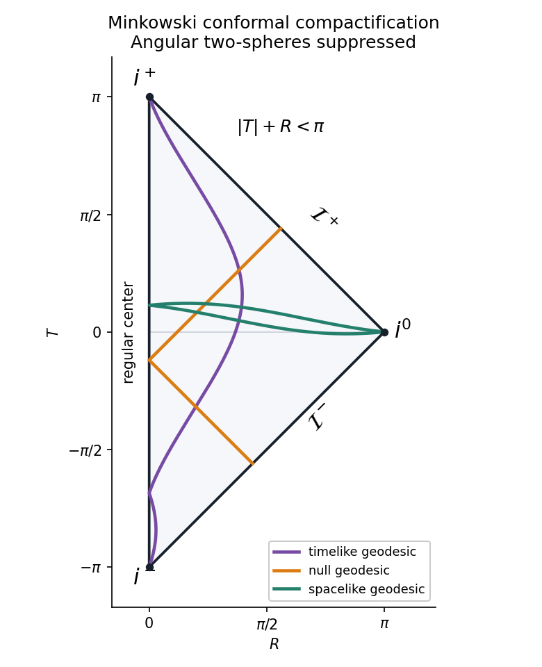
Minkowski conformal compactification and the endpoints of timelike, null and spacelike geodesics
. Details. 
The original Penrose diagram suppresses the angular spheres. The displayed physical paths illustrate their distinct endpoint types; the two sloping boundaries are null infinity, while the left edge is the regular center.
Articles by others on the same topic
There are currently no matching articles.