For an ideal gas with constant adiabatic index , let and be specific heat capacities and . The ideal gas law and the internal energy of an ideal gas give and specific internal energy . Since , the internal energy per unit volume is . Consequently a star with spherical symmetry hasThe radial integral requires the volume measure : the first printed expression omits this factor if its differential is read literally as . The mass-coordinate expression confirms the required volume interpretation.
Define the enclosed mass , total mass and dimensionless shell label . Mass conservation gives , so the change of variables givesHere labels a fixed material shell rather than its radial position. In a mass-preserving stellar homology, with . Both a shell's radius and thickness gain a factor , so its volume gains and its mass density becomes . An adiabatic process keeps fixed separately in each shell, even if that constant differs between shells. Thus and . Integration at fixed mass labels provesThe spherical shell theorem gives the Newtonian gravitational potential energy by assembling shells against the mass already inside them:Every radius gains the same factor , while and remain fixed. HenceThis is the homologous adiabatic stellar stability test. The derivative with respect to the physical stellar radius is . Stationarity at therefore requires , orAfter imposing this equilibrium relation, andSince , a strict energy minimum under this homologous displacement requiresFor , contraction sends to , expansion sends it to from below, and is the unique minimum, with . For , contraction sends to , expansion sends it to from above, and is the unique maximum. When , the equilibrium relation makes for every : the scale direction is marginal, not strictly stable. The plotted curves display these three possibilities. This checks homologous radial stability; stability against every stellar displacement needs a fuller perturbation analysis.
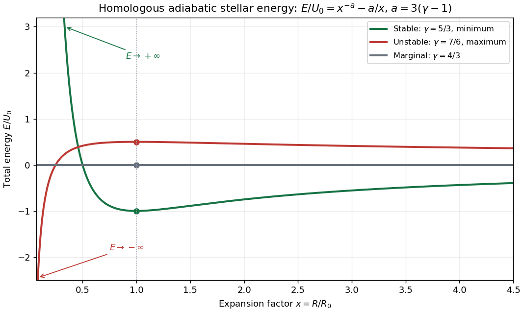
Stellar energy under homologous adiabatic expansion: stable minimum, unstable maximum and marginal scaling
. Details. 
Write for the one-dimensional thermal velocity dispersion of an isotropic monatomic ideal gas. An isothermal process keeps fixed, and the vertical pressure is . Hydrostatic equilibrium in the Newtonian gravitational potential givesPlanar symmetry reduces the Poisson equation for Newtonian gravity to . Combining the two equations yieldsThe velocity factor here is a velocity second moment, not the square of a particular particle's instantaneous vertical velocity.
Set and try the symmetric self-gravitating isothermal slab profile . Its logarithmic derivatives areThe chosen makes the second expression satisfy the required equation. The central conditions and fix the smooth even solution uniquely. In the scale-height convention used here,The undefined constant printed as in the scale-height denominator must be ; this follows both from substitution and dimensions.
Integrating hydrostatic equilibrium, with the additive potential constant chosen so that , givesThe orbits in a self-gravitating isothermal slab separate into horizontal and vertical motions. There is no horizontal force, so and , with constant horizontal velocities. For collisionless test particles, or between gas collisions, conservation of energy fixes the vertical energyEvery finite has two turning points , whereThus the general orbit drifts uniformly in the plane while oscillating periodically across it. A particle with stays in the midplane; an orbit with nonzero horizontal velocity is generally not closed.
Near the plane, , so the vertical motion is a harmonic oscillator with . Far from the plane, and the force tends to a constant magnitude. Indeed the surface density is , and that magnitude is . Large-amplitude vertical motion is therefore approximately uniformly accelerated on each side, rather than sinusoidal. Because this ideal slab extends infinitely in the horizontal directions and its potential grows without bound as , no finite-energy particle escapes vertically.
For an isolated smooth mass distribution with spherical symmetry, assemble each shell at radius against the Newtonian gravitational potential of its interior mass. The spherical shell theorem givesAssume finite total mass, finite binding energy and no central point-mass self-energy, so vanishes at both endpoints. Integration by parts then givesFor example, near a regular center guarantees the central boundary condition, while finite total mass guarantees the one at infinity. A divergent central binding energy would fall outside this formula's finite-energy hypotheses.
For the discrete system use the centre of mass frame, let be the particle number, and write . The printed in the particle-count factor and the subsequent must be understood consistently as . DefineBy Newton's second law, differentiation givesEach pair contributesTherefore the exact dynamical virial theorem is . In a stationary statistical state, or on a bounded-motion time average for which the mean vanishes, it becomesThere is no external pressure, tidal field or boundary work in this isolated point-particle derivation. For a time-averaged system, the following and gravitational radius refer to that same averaged binding energy.
Using and , virial equilibrium givesThis is the three-dimensional mean squared speed about the centre of mass. For an isotropic system each one-dimensional velocity dispersion squared is one third of it.
Set the Newtonian gravitational potential to zero at infinity and exclude each particle's own field. The local escape velocity in the instantaneous frozen potential obeys , where . Since every pair occurs twice, . Averaging over the identical particles proves the gravitational rms escape and collapse speeds relationAn actual encounter in a changing potential can exchange energy, so this is the usual local escape-speed definition, not a claim about every many-body trajectory.
Finally, dissipation-free collapse from rest at infinite separation has total energy zero. Conservation of energy at the specified binding energy therefore gives , twice the equilibrium kinetic energy at the same . HenceThis mean squared speed includes coherent infall; a local random velocity dispersion after subtracting the infall velocity need not obey that ratio.
There is a genuine inconsistency in this part. For any nonnegative metallicity distribution function, its maximum is at least its mean. A population of positive mean solar metallicity cannot have a maximum equal to half that mean. For example, a uniform abundance distribution on has mean and maximum . Thus the printed maximum-to-mean ratio cannot be proved. The following calculation explains the supplied function, gives the consistent distribution, and also treats the literal birth-metallicity interpretation separately.
Let denote the supplied abundance function. Algebraically it isWith , a Taylor series of givesConsequentlyThis is an early-consumption expansion: its fractional correction is . Small yield alone does not make the expression linear throughout most of the gas-consumption history. At fixed , the small- expansion instead is
In a well-mixed closed-box model of galactic chemical evolution, the gas fraction of a galaxy also labels the permanently locked stellar mass: . Newly formed stars inherit the current gas-phase metallicity . Therefore the mass-weighted mean stellar metallicity satisfies the cumulative and birth stellar metallicities relationApplying the derivative to givesThus the supplied function has the natural interpretation of a cumulative mean, not an individual star's birth abundance. Direct integration of verifies that it gives exactly . This is the saturating closed-box enrichment law: it corresponds to effective stellar yield , with measured as a fraction. The usual constant-yield trace-metal model instead gives . Both agree to first order when ; their exact formulae should not be identified outside that regime.
Let the final gas fraction be and . In the consistent mean-metallicity interpretation, while the most recently formed stars have the maximum . At early consumption,so the corrected result isThe assumption here includes , equivalently in this approximation. Exactly, and determine the maximum implicitly; it remains larger than the mean, but its ratio to the mean need not equal two after substantial consumption.
For the mass-weighted metallicity distribution function, stars formed while the gas fraction falls by have probability . Writing their individual abundance as gives and the change of variablesThe density is zero outside this interval. Its cumulative probability is , so it integrates to one; integrating reproduces . A star-count distribution has the same form if the initial mass function and survival selection give a fixed number of observed stars per unit locked mass. Luminosity-weighted samples require different weights.
For trace abundances, to leading order at fixed . The corresponding ordinary closed-box metallicity distribution isIn the early-consumption regime , this becomes approximately uniform, on . Its mean is half its upper endpoint, again producing the corrected maximum .
If the supplied is instead retained literally as the individual birth abundance, set rather than . The observation-time population mean is then , not . Its exact distribution can be specified parametrically usingPositivity follows because is the average of the increasing function . Its support is , and normalization follows directly from . At early consumption it is uniform with , maximum and mean . Even this literal alternative gives maximum twice the population mean, never half. The distinction between birth abundance and cumulative mean resolves the calculation; the printed inverse maximum-to-mean ratio is false under either interpretation.
Articles by others on the same topic
There are currently no matching articles.