Write for two rows of the data matrix and . Three possible dissimilarities for continuous variables are the following.
The Euclidean distance isIt is simple and has the usual geometric interpretation when coordinates have comparable units. Its disadvantage is sensitivity to the numerical scales: a change of units or a high-variance variable can dominate it. Strongly correlated coordinates can also give repeated weight to essentially the same information. Squared Euclidean distance is useful in some methods, but is not itself a metric because it need not satisfy the triangle inequality.
The standardized Euclidean distance iswhere is the sample variance of coordinate across individuals. It measures differences in standard-deviation units and is invariant under positive coordinate rescalings when the scales are estimated consistently. It is useful for differently measured variables, but requires nonzero sample variances, ignores correlations between coordinates and can give excessive influence to a low-variance noisy variable. With fixed positive scales it is a Euclidean distance after a diagonal change of coordinates, so it is a metric.
The Mahalanobis distance iswhere is the pooled sample covariance matrix of all individuals. If is its Cholesky decomposition, then : it is Euclidean distance in whitened coordinates. It adjusts for both scales and correlations, avoiding duplicate weight for highly correlated variables, and is invariant under nonsingular affine transformations when the sample covariance matrix is transformed accordingly. No multivariate normal distribution assumption is required merely to define the distance. However, must be a positive-definite matrix; when there are too few observations or dependent coordinates, its inverse is unavailable. Estimation of can also be unstable and sensitive to outliers. These trade-offs determine whether covariance adjustment is preferable to the simpler distances.
A metric dissimilarity must satisfy nonnegativity, separation, symmetry and the triangle inequality:The underlying objects must be specified: here they are binary measurement profiles, rather than labels attached to individuals.
Let count coordinate pairs of the indicated types. The simple matching coefficient is , so its complementary dissimilarity is . Counting mismatches in every pair gives the dissimilarity matrixFor the Jaccard coefficient, joint absences are excluded: . Thus the Jaccard distance is , givingOnly the pair of individuals two and four has a joint absence. Their profiles have one shared presence, two mismatched presences and one joint absence, giving dissimilarities and , respectively. All other pairs have a presence in at least one profile at every coordinate, so the two denominators coincide.
For the requested metric property of simple matching dissimilarity, write a general pair of -coordinate binary profiles as . Thenwhich is the normalized Hamming distance. It is nonnegative and symmetric, and equals zero exactly when all coordinates match. For each coordinate, a mismatch between and forces a mismatch between or between . ThereforeSumming and dividing by proves the triangle inequality, establishing all four metric properties. Simple matching dissimilarity is a metric on binary profiles. If two separately labelled individuals have identical profiles, it gives zero distance between them, so on those labels it is only a pseudometric. The four profiles here are distinct, so this distinction does not prevent from defining a metric on the given sample.
There is a defect in the stated geometric interpretation of the data. The supplied numbers cannot be Euclidean distances, becauseThey violate the triangle inequality; independently, . Nevertheless, both clustering algorithms are defined for this symmetric dissimilarity matrix. The calculations below retain the supplied numbers and use agglomerative clustering of nonmetric dissimilarities, rather than silently inventing Euclidean replacement data.
In single-linkage clustering, the intercluster dissimilarity isThe closest pair is , merging at . Among the remaining clusters the next closest pair is , merging at . The three intercluster dissimilarities are nowConsequently merges with at , using the cross-pair . The remaining point joins at , using . The dendrogram thus hasThe close pairs and are the clearest early groupings. A cut between and produces these two pairs and the singleton ; a cut between and produces and . Single-linkage clustering builds chains through close cross-pairs, so the merge at does not mean every pair in is that close: . The data alone do not prescribe a unique number of clusters.
For complete-linkage clustering, replace the minimum by the maximum:The first two merges remain at and at . SubsequentlyThus joins at . The final maximum between and is , givingBoth the topology and the later heights of the dendrogram change: complete-linkage clustering attaches to before joining that group to , rather than merging the two pairs first. Its control of the largest within-cluster separation makes it less susceptible to the chaining seen with single-linkage clustering.
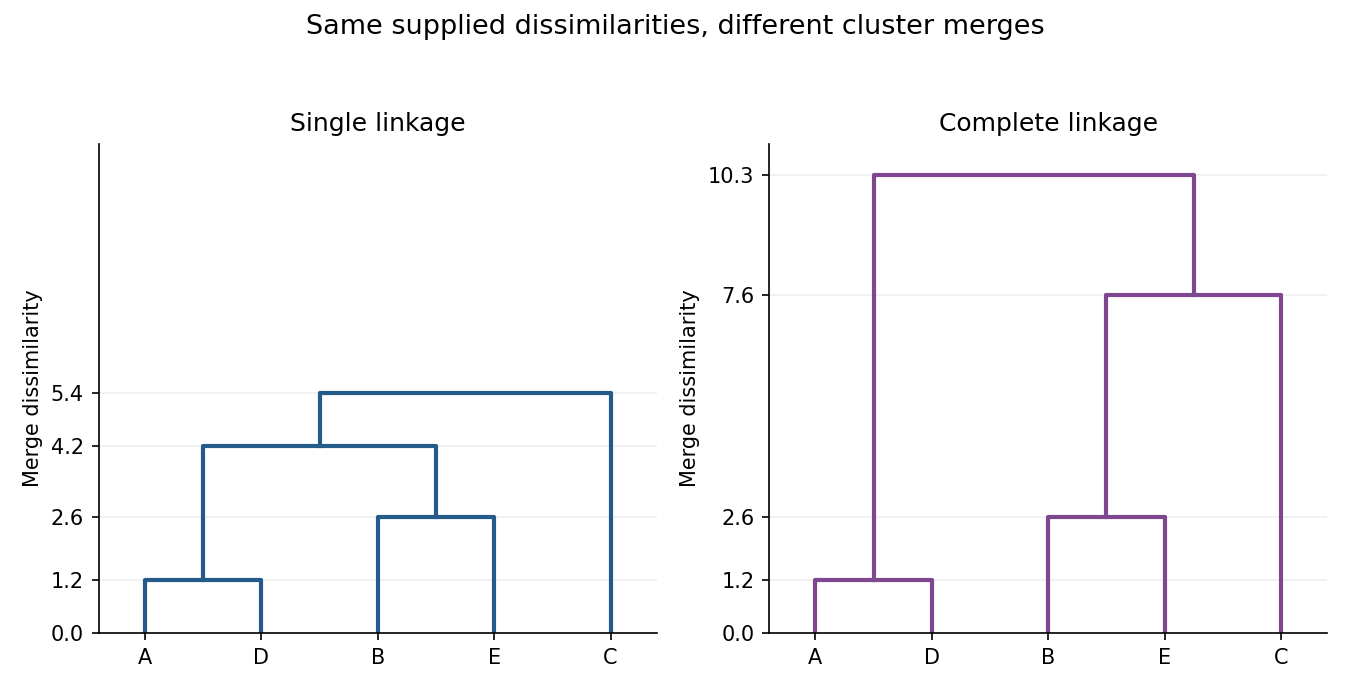
Single-linkage and complete-linkage dendrograms for the supplied five-subject dissimilarities
. Details. 
Articles by others on the same topic
There are currently no matching articles.