The linear damped harmonic oscillator has characteristic exponents . Imposing both initial conditions gives, for ,For completeness, at its continuous limiting form is ; for replace by . The initial derivative is one, as the original PDF specifies; the converted TeX loses this derivative and corrupts the time derivatives in both oscillator equations.
The separate nonlinear oscillator has quadratic drag. Introduce the slow time and use the method of multiple scales,The order- equation isFor positive amplitude, write . Its right side is . The cosine coefficient of the last angular function iswhile its sine coefficient is zero. The solvability condition in the method of multiple scales removes the resonant harmonics, givingThe leading initial conditions select , . Therefore the quadratically damped oscillator hasThe same sign follows from the exact energy balance . Averaging gives , consistent with the amplitude equation.
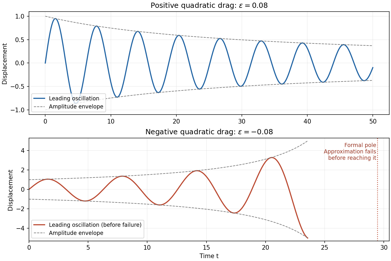

For , the amplitude decays algebraically and stays at most one. On each fixed interval , the omitted displacement correction is , so this approximation is valid through times of order . The effective drag strength decreases rather than increases, and the envelope predicts at later times. There is no finite-time pole in the positive-drag approximation. A uniform error assertion for arbitrarily long intervals is stronger than the finite-slow-time expansion just derived; the stated estimate applies to the specified range.
For , write . The amplitude grows as , with a formal pole atOn fixed slow-time intervals strictly before that pole, the displacement error remains . This estimate is not uniform as : nonresonant corrections have size comparable to , and the required weak-drag condition is . Thus the approximation necessarily fails when , corresponding to a distance of order one in fast time from the formal pole, and may require additional error control when approaching it. The plot therefore stops short of the pole. Its position is a prediction of the leading amplitude equation, not an exact blow-up time for the original nonlinear equation; continuing the formula past it is invalid.
At fixed , expand the exact damped harmonic oscillator solution using , and . Its Poincaré expansion through first order isThe correction is a secular term. When is order one it is not small, and the truncated amplitude eventually changes sign and grows in magnitude, instead of reproducing positive damping. This loss of ordering is why a fixed-time regular perturbation is unsuitable on the damping timescale.
Retain the exact damping factor and expand only the slowly accumulating phase. With bounded,The resulting two-time expansion of a weakly damped linear oscillator isIn slow-time notation the second term in parentheses is , an order- correction. Simply retaining would have order- rather than order- error on this scale, and would not meet the requested accuracy.
When , the phase shift is order one: Taylor-expanding its sine and cosine is no longer an ordered asymptotic expansion of the oscillatory factor. The exact solution and acquire visibly different phases after removing their common exponential damping. In contrast, for the main difference between and is their amplitude envelope: versus .
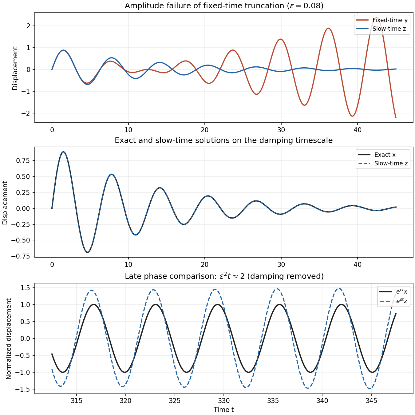
Fixed-time and slow-time linear oscillator approximations, with a damping-normalized late-time phase comparison
. Details. 
The phrase “not valid” on the later scale needs an error convention. For fixed positive damping, the absolute displacement of both and is exponentially small when is a positive order-one number. Indeed Taylor's theorem gives, for small positive ,The supremum of the right side over is . Thus loses phase accuracy on , but does not lose an absolute error bound there. The last plot displays and to show that phase failure honestly; multiplying by the damping factor would make the difference extremely small. Relative pointwise error also becomes singular near zeros, so accuracy of the oscillatory factor is the meaningful late-time comparison.
Articles by others on the same topic
There are currently no matching articles.