Quadratic drag

Quadratic drag has magnitude proportional to the square of the relative speed and points opposite to the relative velocity.

For an isotropic model of a body of fixed shape, let $\mathbf{U}={\mathbf{v}}_{\mathrm{body}}-{\mathbf{u}}_{\infty }$ denote its relative velocity through the distant fluid, with $U=|\mathbf{U}|$. A constant positive resistance $k$ givesHere density $\rho$, reference area $A$ and drag coefficient $C_D$ are held fixed over the modeled range of relative speeds. The vector formula makes the direction explicit: the drag force on the body opposes its motion relative to the fluid, and vanishes at $U=0$. For a general body, orientation and other flow conditions can affect the drag coefficient; treating it as a constant requires a regime in which that is an adequate approximation. ^[ref]

Compare two distinct models at a chosen relative speed $U_0>0$. A linear drag model has $F_D(U)/F_D(U_0)=U/U_0$, while a constant-coefficient quadratic drag model has $F_D(U)/F_D(U_0)=(U/U_0{)}^2$. At $U=2U_0$ their drag force ratios are two and four respectively.

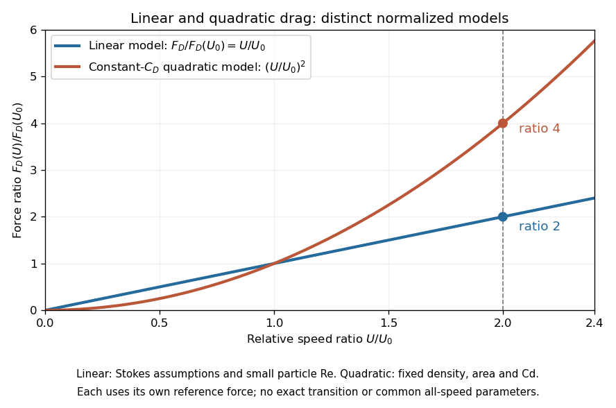
This distinction matters when estimating terminal velocity or trajectories such as descent from rest under quadratic drag: doubling relative speed increases the resistance much more strongly in the quadratic drag model. An approximately constant drag coefficient can occur in another Reynolds number regime; its use must be justified there. Conversely, substituting the creeping-flow sphere coefficient $C_D=24/{\mathrm{Re}}_d$ into $F_D=\frac{1}{2}\rho U^{2}A{C}_D$ recovers linear drag, so writing this general formula does not make the resistance quadratic. Neither approximation should be extended across all Reynolds numbers.

The distinction already appears in the original investigation underlying the Stokes drag law, read on 9 December 1850: article 42 identifies resistance proportional to relative speed and distinguishes it from a contribution proportional to the square of relative speed. ^[ref]

Let downward velocity $v$ obey $\dot{v}=a-b{v}^2$, with constants $a,b>0$, terminal velocity $v_t=\sqrt{a/b}$ and initial speed $u>v_t$. Gravity minus buoyancy can supply the constant downward force represented by $a$. Since $\dot{z}=v$, the equation for $v^2$ is linear in depth: $d(v^2)/dz=-2b(v^2-v_t^2)$, giving the displayed decay. Exact terminal velocity is approached only asymptotically. A practical tolerance $v\le (1+ϵ)v_t$ is attained at $z_{ϵ}=(2b{)}^{-1}\ln [(u^2/v_t^2-1)/(2ϵ+{ϵ}^2)]$, provided the initial excess exceeds that tolerance. Its time-domain form is $v=v_t\coth (b{v}_{t}t+\chi )$ with $\chi =\mathrm{arctanh}(v_t/u)$, in contrast to the hyperbolic tangent for descent from rest under quadratic drag.

For positive downward speed, gravity and quadratic drag give $m\dot{v}=mg-\alpha v^2$, $v(0)=0$. Separation and the integral of $(1-s^2{)}^{-1}$ give the displayed approach to terminal velocity. The fallen distance is $(m/\alpha )\log \cosh (\sqrt{\alpha g/m}t)$. The limit as $\alpha \to 0$ recovers $v=gt$ and distance $g{t}^2/2$.

For an ice mass in still water, approximate the wind stress by a fixed vector $a{\mathbf{e}}_x$ while retaining quadratic drag in the water. With mass per water-drag area $\mu =m/A_w$, water coefficient $b={\rho }_w{C}_w$ and $f=2\Omega \sin \varphi$, the steady balance is $a{\mathbf{e}}_x=bU\mathbf{u}+\mu f\hat{\mathbf{z}}\times \mathbf{u}$. Resolving along the drift and perpendicular to it gives $a\cos \theta =b{U}^2$, $a\sin \theta =\mu |f|U$. Thus $b^2{U}^4+(\mu f{)}^2{U}^2=a^2$ and $\tan \theta =\mu |f|/(bU)$. The direction is right of the wind in the northern hemisphere and left in the southern hemisphere. This angle neglects intrinsic boundary-layer turning, ocean currents and contact forces; it is not a universal observed sea-ice turning angle.

The normalization $\mu =m/A_w$ has units $\mathrm{kg}{\mathrm{m}}^{-2}$. It converts the Coriolis force into a force per water-drag area and allows comparison with wind and water stresses. Icebergs generally have much larger $\mu$ than thin ice floes, but their effective air-to-water drag-area ratio also matters. A geometric depth becomes a mass per area only after multiplication by density.

A resistive velocity term proportional to the speed squared removes energy at rate proportional to $|\omega {|}^3$. Its derivative at zero velocity vanishes, so it does not appear in the linearization of a dynamical system at rest. Nonlinear energy arguments can still prove asymptotic stability.