Use dominant balance for algebraic roots to separate the three scales. On writing , the equation becomes . Its nonzero simple limiting root is , so one root has .
For the two remaining roots put . Division by gives . The nonzero limiting root is , giving . Finally gives, after division by ,Its simple limiting root is . These three distinct balances account for all roots of the cubic, andFor the root of smallest magnitude, set . The order- coefficient is , so . HenceEach rescaled root is simple at , justifying the regular perturbation of a simple algebraic root rather than treating the original triple root as an ordinary regular perturbation.
The complete integral is . Therefore apply asymptotic expansion by repeated integration by parts to the tail :The last integral is bounded by . ThusIn particular the first three additive terms are , and ; the formula also supplies three successive terms of the exponentially small tail if the constant is counted separately. A power expansion alone would retain only and miss this information.
Take the principal complex logarithm and deform the interval upwards, where decays for . The small indentation at zero contributes nothing because ; the distant horizontal segment vanishes exponentially. The two vertical edges therefore give the exact representationThis is an endpoint steepest descent contour, with distinct contributions from the singular endpoint and the smooth endpoint. Setting in the first integral and using the given logarithmic moment givesFor the second edge, the Taylor series at is . Watson's lemma integrates it term by term as an asymptotic expansion, using . ConsequentlyHere is the Euler--Mascheroni constant. The first smooth-endpoint terms areFor every fixed , retaining leaves . The factorial series is an asymptotic series, not a convergent sum. Treating the logarithmic endpoint by an ordinary smooth-endpoint integration formula would lose the leading logarithm; this is the logarithmic endpoint Fourier asymptotics mechanism.
The linear damped harmonic oscillator has characteristic exponents . Imposing both initial conditions gives, for ,For completeness, at its continuous limiting form is ; for replace by . The initial derivative is one, as the original PDF specifies; the converted TeX loses this derivative and corrupts the time derivatives in both oscillator equations.
The separate nonlinear oscillator has quadratic drag. Introduce the slow time and use the method of multiple scales,The order- equation isFor positive amplitude, write . Its right side is . The cosine coefficient of the last angular function iswhile its sine coefficient is zero. The solvability condition in the method of multiple scales removes the resonant harmonics, givingThe leading initial conditions select , . Therefore the quadratically damped oscillator hasThe same sign follows from the exact energy balance . Averaging gives , consistent with the amplitude equation.
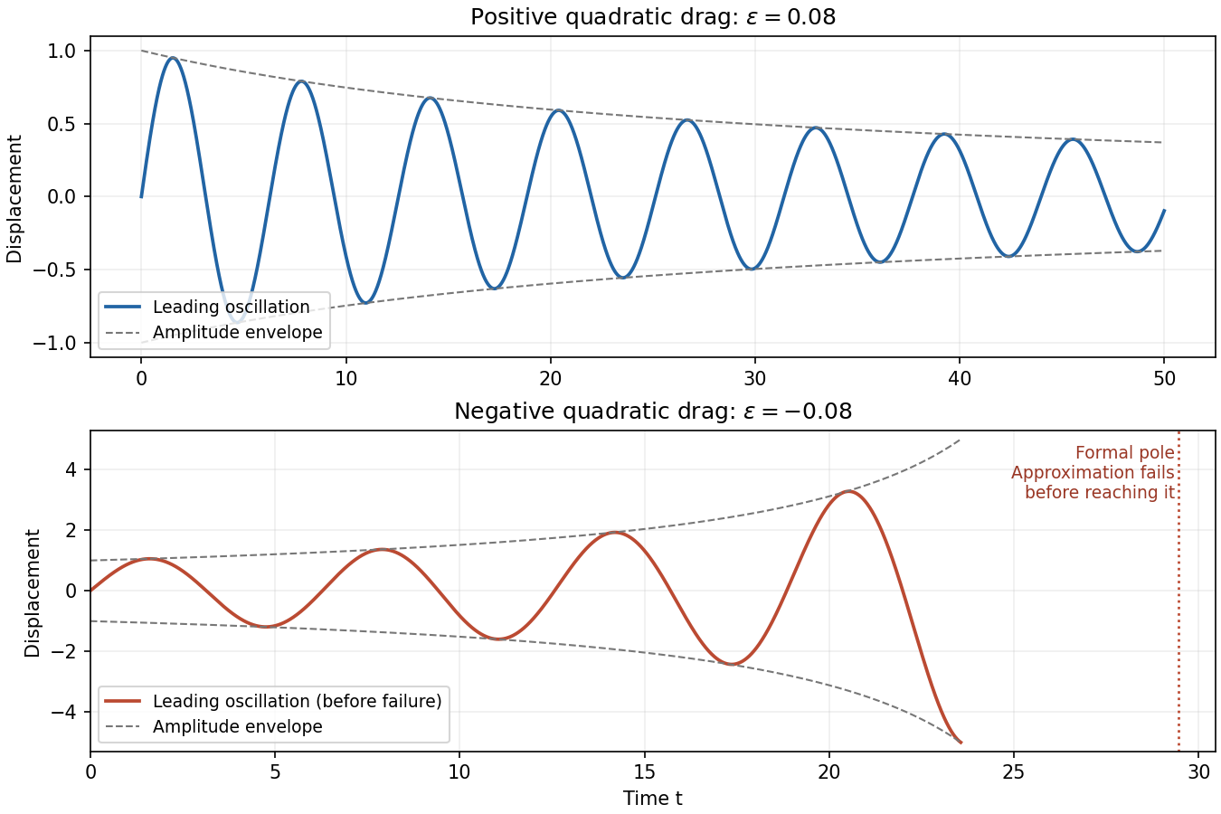

For , the amplitude decays algebraically and stays at most one. On each fixed interval , the omitted displacement correction is , so this approximation is valid through times of order . The effective drag strength decreases rather than increases, and the envelope predicts at later times. There is no finite-time pole in the positive-drag approximation. A uniform error assertion for arbitrarily long intervals is stronger than the finite-slow-time expansion just derived; the stated estimate applies to the specified range.
For , write . The amplitude grows as , with a formal pole atOn fixed slow-time intervals strictly before that pole, the displacement error remains . This estimate is not uniform as : nonresonant corrections have size comparable to , and the required weak-drag condition is . Thus the approximation necessarily fails when , corresponding to a distance of order one in fast time from the formal pole, and may require additional error control when approaching it. The plot therefore stops short of the pole. Its position is a prediction of the leading amplitude equation, not an exact blow-up time for the original nonlinear equation; continuing the formula past it is invalid.
At fixed , expand the exact damped harmonic oscillator solution using , and . Its Poincaré expansion through first order isThe correction is a secular term. When is order one it is not small, and the truncated amplitude eventually changes sign and grows in magnitude, instead of reproducing positive damping. This loss of ordering is why a fixed-time regular perturbation is unsuitable on the damping timescale.
Retain the exact damping factor and expand only the slowly accumulating phase. With bounded,The resulting two-time expansion of a weakly damped linear oscillator isIn slow-time notation the second term in parentheses is , an order- correction. Simply retaining would have order- rather than order- error on this scale, and would not meet the requested accuracy.
When , the phase shift is order one: Taylor-expanding its sine and cosine is no longer an ordered asymptotic expansion of the oscillatory factor. The exact solution and acquire visibly different phases after removing their common exponential damping. In contrast, for the main difference between and is their amplitude envelope: versus .
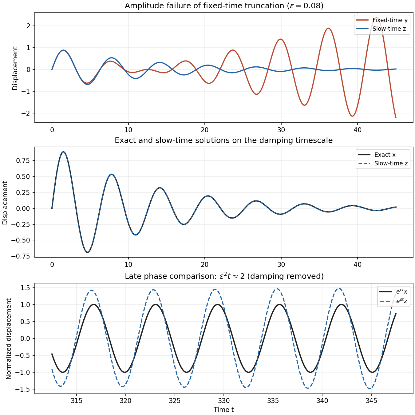
Fixed-time and slow-time linear oscillator approximations, with a damping-normalized late-time phase comparison
. Details. 
The phrase “not valid” on the later scale needs an error convention. For fixed positive damping, the absolute displacement of both and is exponentially small when is a positive order-one number. Indeed Taylor's theorem gives, for small positive ,The supremum of the right side over is . Thus loses phase accuracy on , but does not lose an absolute error bound there. The last plot displays and to show that phase failure honestly; multiplying by the damping factor would make the difference extremely small. Relative pointwise error also becomes singular near zeros, so accuracy of the oscillatory factor is the meaningful late-time comparison.
Multiply the equation by . Its left side is an exact derivative, yielding the first integralFor a solution continuous at the singular endpoint, the limiting value is . This can also be established from the exact integrating-factor formula below, without assuming uniform bounds on derivatives near zero.
Away from zero, the outer expansion has leading term . The endpoint value at one requires if an exponentially amplified homogeneous term is to be avoided. It follows already thatTo exhibit the matching and explain the required boundedness, first set , for a representative without an order-one homogeneous contribution. The leading inner expansion obeysIntegration giveswhere is the exponential integral. For , , matching the outer term . For , , so the intermediate solution behaves as and reaches order one on a second scale .
On this second scale, the first integral becomes, at leading order, . Equivalently its differentiated equation is , as in the hint. The matching solution that tends to zero as isIt has at large , matching the intermediate region, and . Thus the nested layers at an essential singular endpoint connect an order- outer solution to an order-one endpoint value without an unbounded overshoot.
The issue of uniqueness is clarified by exact integration. PutFor every fixed and every prescribed exact value of , the solution satisfying the right endpoint isAs , the integral is asymptotic to , proving . Since , the two exact endpoint values fix the two constants: for a prescribed exact , this finite- boundary-value problem is unique.
However, specifying only the leading value and uniform order-one size does not select a unique asymptotic family. To see this constructively, choose and an arbitrary bounded real constant . WriteThe right endpoint fixesEndpoint Laplace's method gives . Therefore every bounded choice of haswith changes in affecting only by . These solutions are uniformly order one: near zero their particular part has the finite limit , near one it follows the small outer solution, and the freely chosen value at is . The inner-layer homogeneous contribution is also bounded. Indeed vanishes at zero, is order one near , and is exponentially small at one.
Consequently the order-one selected value is , but algebraic asymptotic endpoint data leave an order-one interior freedom. This is beyond-all-orders boundary-value sensitivity. If “constant” were interpreted as fixing exactly and independently of , the omitted algebraic corrections would excite an exponentially large interior homogeneous term; a genuinely uniformly bounded exact family requires the higher-order tuning of . Constancy in does not preclude that parameter dependence.
Use incompressible Euler equations with pressure divided by the constant reference density. Writing , their linearization about the parallel shear flow isTaking the divergence requires the commutator . Both this commutator and the divergence of contribute, so . Applying the Laplacian to givesHence the wall-normal velocity equation isTaking of the streamwise momentum equation minus of the spanwise equation cancels pressure and yields the inviscid Squire equation,This is the vorticity component in the original PDF; the converted TeX corrupts its definition. Impermeable inviscid walls impose . They do not impose a viscous no-slip condition on the tangential perturbation velocity.
For a Fourier mode, set , and . The equations becomeFor Couette flow , , so with . Invert this using the Dirichlet Green function of on . If and , it isIt vanishes at both walls and its first derivative has jump one at . ThusAt , uniqueness of the Dirichlet inversion recovers the compatible initial velocity. This inviscid Couette initial-value Green function directly solves the initial-value problem without a Laplace transform.
The Squire equation is now a first-order forced equation in time. Its integrating factor givesFor nonzero , the velocity formula contains shearing phases and the inviscid Couette continuous spectrum. Velocity cancellation can occur even though the transported has constant magnitude; it must not be confused with exponential modal instability.
For the separate case , , the Dirichlet operator is invertible and . Hence andSince in this case, . This is the lift-up effect: a transverse disturbance transports base-flow momentum and creates a streamwise perturbation growing linearly in time, with perturbation kinetic energy generically growing as . The growth is algebraic and is possible without an exponentially unstable normal mode. For nonzero initial normal velocity and nonzero shear, nonlinear effects eventually limit the validity of the linearized calculation. The same streamwise-independent result holds with replaced by for a general parallel profile.
Let and suppose a growing normal mode has , taking without loss of generality. Since never vanishes on the real channel, choose a continuous square-root branch and write . Direct differentiation givesSubstitution into the Taylor–Goldstein equation and division by givesThus the required transformation isThe impermeable walls give , hence . Multiply by , integrate across the channel, and use integration by parts. With the boundary term zero, the resulting power-transformed Taylor–Goldstein energy identity isBoth and are real. Since and , its imaginary part, divided by , isIf everywhere, the integrand is nonnegative and the first two terms have positive integral for any nonzero mode. This contradicts the identity. Therefore instability requiresThis is the necessary instability condition of the Miles–Howard theorem. Where , it says that the gradient Richardson number must be below somewhere. It is not a sufficient condition for instability, and the conclusion concerns exponential normal-mode growth, not exclusion of the algebraic lift-up effect in part (a). The algebra uses the given nondimensional ; in dimensional notation its counterpart is the squared buoyancy frequency.
Articles by others on the same topic
There are currently no matching articles.