Past exam of the mathematics course of the University of Cambridge / 2009 / iii / Paper 48 (Advanced Quantum Field Theory)

Use position eigenstates normalized by $⟨q|q^{\prime }⟩=\delta (q-q^{\prime })$, and the free Hamiltonian operator $\hat{H}={\hat{p}}^2/(2m)$. The time-sliced path integral is the matrix element of the time-evolution operator:Insert momentum eigenstates, with $⟨q|p⟩=(2\pi \hslash {)}^{-1/2}{e}^{ipq/\hslash }$. The free-particle propagator becomesComplete the square in the exponent:The Fresnel integral, defined by the damping prescription $T\to T-i0$, gives, for $T>0$,The square-root branch is $i^{-1/2}=e^{-i\pi /4}$; it is fixed by the regulated Gaussian integral and the short-time Dirac delta distribution limit, rather than an arbitrary phase.

The Euler-Lagrange equation for the free particle is $m\ddot{q}=0$. Its unique classical path satisfying the endpoint boundary conditions is $q_{\mathrm{cl}}(t)=q^{(i)}+\Delta qt/T$. Therefore its classical action isSubstituting into the operator result yields $\mathcal{I}=C(T)e^{i{S}_{\mathrm{cl}}/\hslash }$, with $C(T)=(m/(2\pi i\hslash T){)}^{1/2}$ independent of the endpoint positions.

The same independence is transparent directly in the path integral. Write $q=q_{\mathrm{cl}}+\eta$, with $\eta (0)=\eta (T)=0$. The cross term in the action is $m{\dot{q}}_{\mathrm{cl}}{\int }_0^T\dot{\eta }dt=0$, so $S[q]=S_{\mathrm{cl}}+(m/2){\int }_0^T{\dot{\eta }}^{2}dt$. The fluctuation integral depends only on $m,T,\hslash$. Because the action is quadratic, the factorization is exact; the semiclassical propagator already equals the full answer.

Put $I_0=\sqrt{2\pi /m^2}$ and assume $m^2>0$. The normalized free Gaussian integral has covariance $\Delta =1/m^2$. Expanding the interaction exponential and using Wick's theorem gives the Feynman rules: a quartic vertex contributes $-\lambda$, each internal propagator contributes $\Delta$, and each vacuum diagram is divided by its Feynman-diagram symmetry factor. Multiply the resulting sum by $I_0$. Because we are expanding $I$, rather than $\log I$, disconnected vacuum diagrams must also be included.

At order ${\lambda }^2$ there are two quartic vertices and four internal propagators. Let $r$ be the number of edges joining the two vertices. The remaining half-edges must pair at their own vertex, so $r$ is even. The possibilities $r=0,2,4$ exhaust the vacuum diagrams:

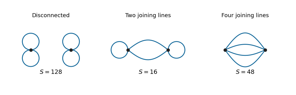
For $r=0$, each vertex has three possible pairings, giving $N_0=9$ Wick contractions. For $r=2$, choose the two half-edges at each vertex, then pair the chosen half-edges across the vertices: $N_2={\left(\genfrac{}{}{0ex}{}{4}{2}\right)}^{2}2!=72$. The remaining two half-edges at each vertex form a self-loop. For $r=4$, all half-edges pair across the vertices, giving $N_4=4!=24$. The common denominator from the expansion is $2!(4!{)}^2=1152$, so the Feynman-diagram symmetry factors areEach vacuum diagram has the same factor $I_0{\lambda }^2{\Delta }^4$ before division by its Feynman-diagram symmetry factor. Consequently the coefficient of ${\lambda }^2$ isAs an independent check, the eighth moment obtained from the Gaussian moment pairing theorem is $⟨x^8{⟩}_0=7!!/m^8=105/m^8$, and $105/[2!(4!{)}^2]=35/384$. The first terms of the zero-dimensional quartic perturbation series are thereforeStrictly, the printed phrase “Taylor expansion” means a formal expansion or a right-sided asymptotic expansion. The general coefficient has absolute successive ratio $(4v+3)(4v+1)/[24(v+1)m^4]\to \infty$, so the power series has zero radius of convergence. Nevertheless, for $\lambda \ge 0$ the remainder after any fixed truncation of $e^{-\lambda x^4/4!}$ is bounded by the next absolute term, and its Gaussian integral is finite. This proves the displayed asymptotic expansion as $\lambda \downarrow 0$. For negative real $\lambda$ the defining integral diverges.

The superficial degree of divergence is the power of a common large-momentum scale obtained by scaling all independent internal momenta together, before cancellations or subtraction of divergent subdiagrams. In a scalar field theory with a standard quadratic kinetic term and non-derivative interactions, each loop momentum integral supplies $d$ powers of momentum and each internal propagator supplies minus two. ThusFor a connected Feynman diagram, counting vertex half-edges and applying the stated identity for the loop order givesIt follows that $D=(d-2)L-2V+2$. Meanwhile, ${\sum }_n(n-4)V_n=2I+E-4V=2L-2V+E-2$. Substitution provesThis power counting in quantum field theory concerns the overall scaling: even a Feynman diagram with $D<0$ can contain divergent subdiagrams, and cancellations may improve convergence when $D\ge 0$.

The canonical mass dimensions are $[\varphi ]=(d-2)/2$ and $[g_n]=d-n(d-2)/2$. A finite polynomial scalar field theory has power-counting renormalizability when its interactions have nonnegative mass dimensions and the allowed local counterterms form a finite set closed under subtraction of divergent subdiagrams. For $d>2$, non-derivative interactions therefore satisfy $n\le 2d/(d-2)$. Equivalently,so adding vertices of such interactions cannot force an indefinitely increasing number of external legs or derivatives in divergent counterterms. In dimensions $d\le 2$ a fixed finite polynomial still has this favorable power counting in quantum field theory; the displayed upper bound on $n$ is intended only for $d>2$.

For six-dimensional cubic scalar field theory, $3V=2I+E$ and $L=I-V+1$ yieldThe coupling $g$ has zero mass dimension. The possible overall divergences have $E\le 3$: vacuum energy, a linear tadpole diagram term, a mass term, a kinetic term, and a cubic interaction. These are finitely many local counterterms. Divergent subdiagrams of higher-point Feynman diagrams are removed by the same counterterms, establishing perturbative renormalizability of cubic scalar theory in six dimensions. A real cubic potential is unbounded below, so this claim is one of perturbative quantum field theory, not a claim that the polynomial defines a stable nonperturbative vacuum.

After Wick rotation, use the Euclidean action with positive kinetic and mass terms and interaction $g{\varphi }^3/3!$. The Euclidean momentum-space Feynman rules are: an internal scalar propagator $1/(k^2+m^2)$, a vertex $-g$, momentum conservation at each vertex, integration $d^{6}k/(2\pi {)}^6$ for each independent loop, and division by the Feynman-diagram symmetry factor. Strip the overall momentum-conserving delta function and external propagators when computing an amputated Green's function.

The one-particle-irreducible two-point vertex at one loop is the bubble:

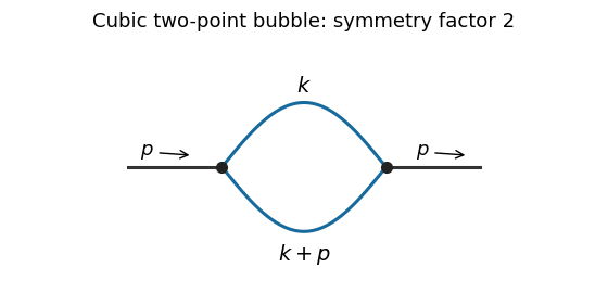
Interchanging its two internal lines is an automorphism, giving Feynman-diagram symmetry factor two. In the normalization of the printed Minkowski amputated Green's function, the two vertices contribute $(-ig{)}^2$, the two internal propagators contribute $(-i{)}^2$, and Wick rotation supplies the overall $i$ already factored out there. Thus the Euclidean bubble contribution isFor this self-energy calculation we impose a vanishing one-point function, so tadpole diagram insertions are canceled by the linear counterterm. Without that convention a connected but one-particle-reducible Feynman diagram with a tadpole insertion is also possible: both external legs attach to one vertex, a zero-momentum line joins it to a second vertex, and that second vertex has a self-loop. Its amputated contribution is $g^2/(2m^2)\int d^{6}k/[(2\pi {)}^6(k^2+m^2)]$, independent of $p$. It is not the bubble drawn above; keeping it without a tadpole subtraction would add this constant to the full amputated answer.

To find the bubble's local divergence, put $K=k^2+m^2$ and expand at large $|k|$:Odd terms vanish under the angular integral. Rotational symmetry gives $⟨(k\cdot p{)}^2⟩=k^2{p}^2/6$. The terms through order $p^2$ are thereforeand the $p^2$ coefficient approaches $-1/(3k^6)$. Terms of order $p^4$ and higher are integrable at infinity in six dimensions; subtracting the two displayed terms leaves an ultraviolet-convergent integral. Hence the divergent part is a local polynomial $A{p}^2+B$, with momentum-independent coefficients. For example, when $m^2>0$ its logarithmically divergent coefficient isChanging the reference scale in this logarithm only changes a finite local term.

At zero external momentum the spherical ultraviolet cutoff and $\mathrm{Vol}(S^5)={\pi }^3$ giveWith $u=k^2$, integrate $u^2/(u+m^2{)}^2=1-2m^2/(u+m^2)+m^4/(u+m^2{)}^2$. This gives the momentum-cutoff two-point function in six-dimensional cubic scalar theoryIn particular, the divergent part of this constant iswhile the last term in $B_{\Lambda }$ tends to a finite constant. For $m=0$ the zero-momentum integral gives $B_{\Lambda }=g^2{\Lambda }^2/(256{\pi }^3)$ directly. The finite parts of a local subtraction can depend on the regularization prescription; the conclusion about mass and kinetic counterterms does not.

Let ${\varphi }_B=Z_{\varphi }^{1/2}\varphi$ define the renormalized field in Phi-fourth theory. For an $n$-point correlation function, with no composite operator insertions, this impliesThe bare correlation function is independent of the arbitrary renormalization scale $\mu$ when the bare parameters and external momenta are fixed. DefineThe definitions of the running mass and wave-function renormalization functions specify their signs and the factor of two. Differentiating $Z_{\varphi }^{n/2}{G}_n$ using the chain rule yields the Callan–Symanzik equationHere ${\hat{\beta }}_{\lambda }$ denotes the renormalization-group beta function itself, not the function multiplied by an additional $\lambda$. The Callan-Symanzik equation concerns dependence on the arbitrary reference scale, with the displayed external momenta kept fixed.

For the minimal subtraction scheme in dimensional regularization, writeso ${\lambda }_B={\mu }^{ϵ}F$ and $m_B^2=m^{2}H$. The ${\mu }^{ϵ}$ factor gives the engineering contribution $-ϵ\lambda$ to the renormalization-group beta function. Put ${\hat{\beta }}_{\lambda }=-ϵ\lambda +{\beta }_{\lambda }$. Scale independence of the bare coupling then givesThe coefficient of ${ϵ}^0$ is $f_1-\lambda f_1^{\prime }+{\beta }_{\lambda }$. Its vanishing proves the first of the simple-pole formulas for minimal-subtraction renormalization group functions:The coefficients of ${ϵ}^{-k}$, $k\ge 1$, also vanish and impose $(\lambda {\partial }_{\lambda }-1)f_{k+1}={\beta }_{\lambda }{f}_k^{\prime }$. These relations explain how the higher poles are consistent with a finite renormalization-group beta function.

For the mass, differentiate the second bare-parameter relation:Its finite coefficient is ${\gamma }_{m^2}-\lambda b_1^{\prime }$. ThereforeThe higher poles impose $\lambda b_{k+1}^{\prime }={\gamma }_{m^2}{b}_k+{\beta }_{\lambda }{b}_k^{\prime }$. The formulas for the running mass and renormalization-group beta function thus follow directly from bare-parameter independence rather than from an identification with diagram coefficients by name.

At the specified loop order, $f_1=3{\lambda }^2/(16{\pi }^2)$ and $b_1=\lambda /(16{\pi }^2)$. There is no wave-function renormalization at this order. HenceThe regulated renormalization-group beta function is ${\hat{\beta }}_{\lambda }=-ϵ\lambda +3{\lambda }^2/(16{\pi }^2)+O({\lambda }^3)$; after removing the regulator, ${\hat{\beta }}_{\lambda }={\beta }_{\lambda }$.

Now take $m^2=0$ and the four-dimensional limit. This massless surface is preserved since $\mu d{m}^2/d\mu =m^2{\gamma }_{m^2}$. Set $b=3/(16{\pi }^2)$, choose a reference scale ${\mu }_0$, and define the running coupling byDifferentiating $1/\lambda$ gives $d(1/\lambda )/d\log \mu =-b$, soThe zero-coupling solution is obtained by continuity. At one-loop accuracy ${\gamma }_{\varphi }=0$, and the chain rule turns the massless Callan-Symanzik equation intoThus the one-loop solution along a running-coupling trajectory isFor a prescribed endpoint coupling $\lambda$, substitute ${\lambda }_0=\lambda /[1+b\lambda \log (\mu /{\mu }_0)]$ on the right. The reference correlation function supplies arbitrary boundary data; the Callan-Symanzik equation determines their scale evolution, not their full momentum dependence. The running coupling formula is used on a branch on which its denominator is nonzero and the retained perturbative approximation is appropriate.

If one keeps $ϵ\ne 0$, the same characteristic calculation uses $d\lambda /d\log \mu =-ϵ\lambda +b{\lambda }^2$. Writing $r=\mu /{\mu }_0$ gives $\lambda (\mu )={\lambda }_0{r}^{-ϵ}/[1-(b{\lambda }_0/ϵ)(1-r^{-ϵ})]$, which tends to the displayed four-dimensional result as $ϵ\to 0$.

With a nonzero anomalous dimension, the characteristic equation instead reads $d{G}_n/d\log \mu =-n{\gamma }_{\varphi }(\lambda (\mu ))G_n$. Integration proves the characteristic solution of the massless Callan-Symanzik equation:For the stipulated ${\gamma }_{\varphi }=c{\lambda }^2$ and the same one-loop renormalization-group beta function, change variables using $d\log \nu =d\lambda /(b{\lambda }^2)$. The exponent's integral becomes $(c/b)(\lambda (\mu )-{\lambda }_0)$. Therefore the modified explicit solution isEquivalently its multiplicative factor is $\exp [-nc{\lambda }_0^2\log r/(1-b{\lambda }_0\log r)]$. This solves the equation with the stated truncated renormalization-group beta function and anomalous dimension; it does not introduce additional higher-order coefficients that were not specified.

A Non-Abelian gauge theory describes fields with a local redundancy, not an independent physical degree of freedom for each component of its gauge field. Take a compact gauge group with Hermitian generators $T^a$ and Lie algebra structure constants defined by $[T^a,T^b]=i{f}^{abc}{T}^c$. In a mostly-plus metric signature, the pure Yang-Mills theory hasWith the matter gauge covariant derivative $D_{\mu }={\partial }_{\mu }-ig{A}_{\mu }$, a finite gauge transformation acts as $A_{\mu }\mapsto U{A}_{\mu }{U}^{-1}-(i/g)({\partial }_{\mu }U)U^{-1}$. Expanding $U=e^{ig{\omega }^a{T}^a}$ givesThe Yang-Mills action is constant along each gauge orbit. Consequently a naive functional integral $\int \mathcal{D}A{e}^{iS[A]}$ repeatedly integrates the same physical configuration and contains the infinite formal volume of the local gauge group. At quadratic order the same problem appears as noninvertibility: the free kinetic operator annihilates $A_{\mu }={\partial }_{\mu }\omega$, so no unique gauge-boson propagator exists. In canonical language the Gauss law constraint in gauge theory and the absence of an independent momentum for the time component show that the field components cannot all be independent oscillators. In covariant quantization, time-like and longitudinal polarizations must not be counted as additional physical states.

The Faddeev-Popov determinant implements a local quotient by the gauge orbit. Choose $G^a[A]={\partial }^{\mu }{A}_{\mu }^a$ and first impose $G^a[A]=f^a(x)$ for a specified function $f$. This is the Lorenz gauge condition when $f=0$. Its infinitesimal change isThe direct Faddeev-Popov operator is therefore $M_0^{ab}={\partial }^{\mu }(D_{\mu }{)}^{ab}$. Locally, if the condition cuts each orbit once and residual zero modes have been removed by boundary conditions, changing variables from $\omega$ to $G[A^{\omega }]-f$ proves the Faddeev-Popov gauge-orbit identityThe determinant is the functional Jacobian of this change of variables. A finite-dimensional version is $\int d\omega \delta (G(\omega )-f)=1/|\det (\partial G/\partial \omega )|$ near a unique root; the perturbative determinant has a fixed sign or phase, absorbed into normalization. This is the same change-of-variables mechanism used in Bastianelli's derivation of the Faddeev–Popov construction.

Insert the identity into the normalized functional integral for a gauge-invariant observable $\mathcal{O}[A]$:For each fixed $\omega$, change the integration variable from $A$ to $A^{\omega }$. The action, observable and measure are invariant, and the determinant is the orbit Jacobian at the resulting gauge slice. The integrand is now independent of the separately integrated orbit parameter. Its integral is $\mathrm{Vol}\mathcal{G}$, canceling the denominator. Thus, up to normalization,This assumes an anomaly-free measure and a local perturbative gauge slice; it is not an assertion of a globally unique representative on every gauge orbit.

Average over $f$ with weight $\exp [-i\int d^{4}x{f}^a{f}^a/(2\xi )]$. The delta functional sets $f=G[A]$, so the average produces the covariant gauge termNext represent the Faddeev-Popov determinant by a Grassmann Gaussian integral. Choose $M=-M_0=-{\partial }^{\mu }{D}_{\mu }$; changing $M_0$ to $-M_0$ changes the regulated determinant by a field-independent factor that is absorbed in normalization. For a Faddeev-Popov ghost field $c$ and independent antighost field $\bar{c}$,To see why it is a determinant rather than its reciprocal, diagonalize a finite-dimensional quadratic form formally: for each Grassmann pair only the term proportional to ${\bar{c}}_j{c}_j$ survives integration, supplying one eigenvalue. Multiplying the surviving eigenvalues gives $\det M$, with an overall factor of $i$ per pair. The functional version is defined with the same regulator as the rest of the theory.

Combining these steps gives the gauge-fixed Yang–Mills LagrangianThis is the gauge-fixed Yang-Mills Lagrangian in a covariant gauge. Integrating its ghost term by parts givesThe second term is the ghost-gluon vertex in the antighost convention chosen here. The Faddeev-Popov ghosts are anticommuting Lorentz scalars introduced to represent a determinant; they are not extra asymptotic particles. A closed ghost loop has a minus sign from their Grassmann parity. In a Non-Abelian gauge theory the determinant depends on $A$, so these loops are essential. In an Abelian gauge theory $D_{\mu }$ in the adjoint sector reduces to ${\partial }_{\mu }$, the determinant is field independent, and its ghost sector decouples.

The quadratic gauge field kernel at non-null momentum isDefine the mixed-index longitudinal projector of a vector field $P_L{}^{\mu }{}_{\nu }=k^{\mu }{k}_{\nu }/k^2$ and transverse projector of a vector field $P_T=1-P_L$. The kernel is $-k^2(P_T+{\xi }^{-1}{P}_L)$ and hence has inverse $-k^{-2}(P_T+\xi P_L)$. Multiplying by $i$ gives the gauge-boson propagator, off its poles,The vacuum Feynman i-epsilon prescription completes this off-pole formula; with the mostly-plus convention its physical transverse denominator is $k^2-i0$. The choice $\xi =1$ is Feynman gauge; $\xi \to 0$ is covariant Landau gauge. The invertible quadratic kernel supplies perturbation theory, while the ghost determinant ensures the gauge-orbit measure has been accounted for.

The consistency of the unphysical sector is organized by BRST symmetry. Introduce a bosonic Nakanishi-Lautrup field $B^a$ and a left-acting BRST differentialThe graded Leibniz rule and the Jacobi identity give $s^2=0$: for example $s^{2}A=D(sc)+g[Dc,c]=0$ since $D[c,c]=2[Dc,c]$, and $s^{2}c$ vanishes by the graded Jacobi identity. Nilpotence on $\bar{c}$ and $B$ is immediate. Using the odd antighost field, the same graded Leibniz rule givesEliminating $B^a$ by its algebraic field equation $B^a=-G^a/\xi$ recovers the displayed gauge-fixing and ghost terms. Thus they are BRST-exact together, and the total action preserves BRST symmetry. At the level of states, the BRST charge $Q$ implements physical states as the ghost-number-zero BRST cohomology $\ker Q/\mathrm{im}Q$. This prescription removes longitudinal, time-like and ghost excitations from physical amplitudes while allowing them on internal lines. For a BRST-closed observable, changing $\xi$ inserts $s({\bar{c}}^a{B}^a/2)$; its expectation vanishes by the BRST change-of-variables identity when the measure preserves the symmetry. This explains the independence of physical quantities from the arbitrary gauge parameter.

Finally, a local condition such as Lorenz gauge can have several solutions on the same gauge orbit, the Gribov ambiguity. The preceding Faddeev-Popov gauge-orbit identity and perturbative gauge fixing construction apply in a neighborhood where the linearized operator is invertible after residual modes are excluded. They resolve perturbative gauge overcounting and supply consistent covariant Feynman rules; they do not by themselves prove a globally unique nonperturbative gauge fixing.