Past exam of the mathematics course of the University of Cambridge / 2010 / iii / Paper 50 / 1

The density operators are Hermitian, so their squared Hilbert-Schmidt distance is $2V=\mathrm{Tr}({\rho }^2)+\mathrm{Tr}({\rho }_d^2)-2\mathrm{Tr}(\rho {\rho }_d)$. Both purity of a density operator values are constant under their respective unitary time evolution: cyclicity gives $\mathrm{Tr}(\rho [H,\rho ])=0$ for every Hermitian $H$. ConsequentlyThe terms containing $H_0$ cancel because $\mathrm{Tr}([-i{H}_0,\rho ]{\rho }_d)=-\mathrm{Tr}(\rho [-i{H}_0,{\rho }_d])$. The quantity $F=\mathrm{Tr}({\rho }_d[-i{H}_1,\rho ])$ is real: $[-i{H}_1,\rho ]$ is Hermitian, and the trace of the product of two Hermitian matrices equals its conjugate. The Lyapunov quantum control choice $f=F$ therefore gives $\boxed{\dot{V}=-f^2\le 0}$. For $t_2\ge t_1$, integration yields $V(t_2)=V(t_1)-{\int }_{t_1}^{t_2}f(t{)}^{2}dt\le V(t_1)$. Since the distance is $\sqrt{2V}$, it is monotonically nonincreasing. The decrease need not be strict when $f=0$.

Neither monotonic decrease alone nor equality of the initial spectra guarantees convergence. A nonnegative Lyapunov function can approach a positive limiting value, and the set where $\dot{V}=0$ can contain trajectories other than the target. Different initial spectra already obstruct exact tracking: unitary time evolution preserves the eigenvalues of each density operator, while two matrices approaching one another in norm must have the same limiting eigenvalues.

Even the spectral obstruction can be absent while the Lyapunov quantum control stalls. Take a qubit with $H_0=Z/2$, $H_1=X$, ${\rho }_d(0)=|0⟩⟨0|$ and $\rho (0)=|1⟩⟨1|$. Both density operators commute with $H_0$, and the commutator of $X$ with $\rho$ has zero diagonal, so $f=\mathrm{Tr}({\rho }_d[-iX,\rho ])=0$. Both states remain constant. They have the identical spectrum $(1,0)$, but $\boxed{\Vert \rho (t)-{\rho }_d(t){\Vert }_{\mathrm{HS}}=\sqrt{2}\text{ for all }t}$. Moreover $iZ,iX$ generate the full special unitary Lie algebra $\mathfrak{su}(2)$, so the failure here is a limitation of this particular feedback law, not a lack of available state-transfer controls.

The Lyapunov quantum control law requires an exact instantaneous expectation value. Cyclicity writes it aswhere $A(t)$ is a known Hermitian observable. A measurement on one system produces a random outcome, not its exact ensemble expectation, and changes the system state. Repeated measurements for state estimation or continuous weak measurements introduce noise and backaction absent from the assumed closed-system equation. Thus the law cannot be implemented unchanged as exact measurement-based quantum feedback while retaining the dynamics and guarantee in part (a). A conditional-state feedback scheme must include the measurement evolution and rederive its stability properties.

If the initial density operator and Hamiltonian model are known, we can instead solve the deterministic equations in a computer, calculate $f(t)$ along the simulated trajectory, and apply that precomputed waveform in the laboratory as open-loop control. Ensemble measurements can help calibrate such a waveform, but they do not supply nondisturbing instantaneous feedback from an individual evolving system.

A quantum optimal control problem specifies a terminal task, admissible fields and resource costs. Pure-state transfer can minimize $1-|⟨{\psi }_d|\psi (T)⟩{|}^2$; mixed-state transfer on an accessible spectral orbit can minimize $\Vert \rho (T)-{\rho }_d{\Vert }_{\mathrm{HS}}^2/2$; preparing an observable value can minimize $-\mathrm{Tr}(O\rho (T))$. A gate task can minimize $1-|\mathrm{Tr}(U_d^{†}U(T)){|}^2/n^2$ for an $n$-dimensional Hilbert space, which is insensitive to an overall phase. These different terminal functions encode different tasks even when the dynamics are the same. Fluence penalties, amplitude bounds, bandwidth limits, or the total duration can be added to express experimental requirements.

For example, minimizesubject to $\dot{\rho }={\mathcal{L}}_f(\rho )$ and a specified $\rho (0)$. For a closed system, ${\mathcal{L}}_f(\rho )=-i[H_0+{\sum }_m{f}_m{H}_m,\rho ]$; for an open system add the known Lindblad equation dissipator. Introducing a Hermitian costate $\Lambda$ and taking the Hilbert-Schmidt inner product gives the forward and backward equations and functional gradientFor Hamiltonian controls the second term is $\mathrm{Tr}(\Lambda [-i{H}_m,\rho ])$. The adjoint is defined by the Hilbert-Schmidt inner product; in particular, the closed-system costate equation is $\dot{\Lambda }=-i[H,\Lambda ]$, integrated backward from its terminal condition. An unconstrained interior optimum has zero gradient; amplitude constraints replace this by the corresponding constrained first-order conditions.

Numerically, represent the fields by piecewise constant amplitudes $f_{m,j}$ on slices, or by a finite basis $f_m(t)={\sum }_j{a}_{mj}{b}_j(t)$ such as splines or Fourier modes. For piecewise constant closed-system dynamics, $U_j=e^{-i{H}_j\Delta t}$ and $U(T)=U_K\cdots U_1$. Forward products and backward costates provide all slice derivatives in one pair of propagations. In gradient ascent pulse engineering, update these amplitudes to improve the chosen objective, with projection onto amplitude bounds if needed. The exact slice derivative is the derivative of the matrix exponentialReplacing it by $-i\Delta t{H}_m{U}_j$ is only a short-slice approximation when $H_j$ and $H_m$ do not commute. Other gradient descent or nonlinear optimization methods can optimize the same finite parameter set; direct-adjoint looping avoids a separate dynamical simulation for each control coefficient.

A pulse is accepted after propagation with the actual constrained waveform confirms its terminal error and resource use. Sampling model uncertainties in the objective can favor robust pulses. Nonconvexity means a numerical stationary point need not be a global optimum, so initial guesses, convergence tolerances and a sufficiently resolved time grid matter.

Spectral pulse shaping implements a calculated optical control by modifying its complex frequency spectrum. If the available input pulse has spectrum ${\tilde{E}}_{\mathrm{in}}(\omega )$, program a calibrated mask $M(\omega )=a(\omega )e^{i\phi (\omega )}$ so thatThe temporal waveform follows from Fourier inversion. For a real applied field, its spectrum has conjugate symmetry, so the mask must satisfy $M(-\omega )=M(\omega {)}^{\ast }$. Spectral phase controls interference between frequencies and hence their arrival times, chirp and temporal subpulses; spectral attenuation changes their weights. The optimized field envelope is translated into this complex mask, with compensation for known phase shifts and losses in the optical system.

A typical 4f pulse shaper contains a first diffraction grating, a focusing lens, a mask or spatial light modulator in the common focal plane, a second lens and a second grating. The first grating separates the frequencies by angle. The first lens converts those angles into different transverse positions at the spectral Fourier plane. The pixels of the spatial light modulator modify the amplitude and phase of the corresponding frequency bins. The second lens and grating reverse this spatial dispersion and recombine the components into one shaped output beam. In the ideal symmetric layout the four consecutive propagation distances are $f,f,f,f$, giving the name $4f$.

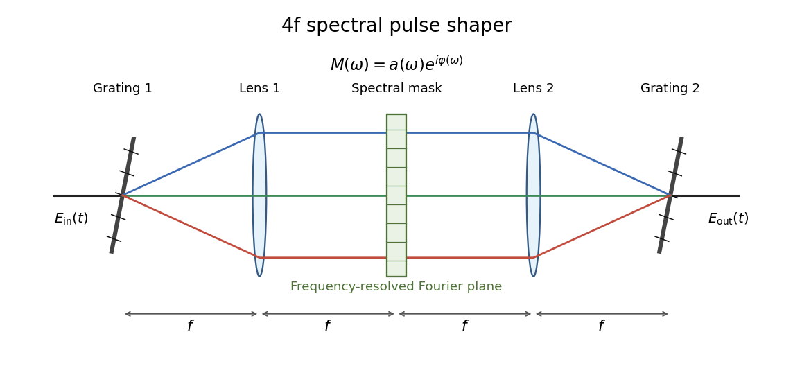
A phase-only spatial light modulator needs suitable polarization optics or another modulation stage for independent amplitude shaping. A passive mask has $0\le a(\omega )\le 1$ and cannot create frequencies absent from the input; finite bandwidth and finite pixel resolution limit temporal features and the useful shaping window. These constraints must be included when converting a mathematical optimum into a laboratory pulse. The programmed mask is an open-loop control, although repeated measurements of the output pulse or system performance can be used to calibrate or optimize it experimentally.