The small root and the root near are regular perturbation roots: they stay finite as the parameter vanishes. Substitution of power series givesFor the third root, dominant balance for algebraic roots requires . The largest terms give , and the missing branch is . The sum of the three roots then yieldsThus the leading roots are , , and ; only the last is a divergent perturbation root. The first regular branch happens to have a zero limit, so retaining its first nonzero term is essential on the long spatial scale.
First take , the decaying half-line regime. If the three exact roots are , the exact initial value problem solution isThis follows either by solving the three initial-value equations or from the Laplace transform . The coefficient formula has sums and .
Retain the three leading roots but compute their coefficients without expanding their denominators. Set , , . A convenient composite asymptotic expansion isIt satisfies all three initial conditions exactly and retains the fast transient, the ordinary decay, and the slow decay. Its first two coefficients are and ; the fast coefficient is . Consequently the simpler bulk expression is , but that expression alone does not reproduce the initial derivative layer.
The absolute error estimate isTo see its uniformity, the slow-root error is , while its magnitude is and its coefficient is . The uniform error bound for nearby decaying exponentials therefore gives an contribution even for . The middle-root error is with coefficient , again giving . The fast-root error is with magnitude and coefficient , giving only . Coefficient errors are or smaller. This estimate concerns itself, rather than asserting the same uniform order for all derivatives or a relative error at its zero.
For the sketch, on one obtainsThus at the origin and rises smoothly after the fast layer. For it rises towards a plateau of height approximately , then decays on the much longer scale . The bulk maximum lies near and has height asymptotic to .
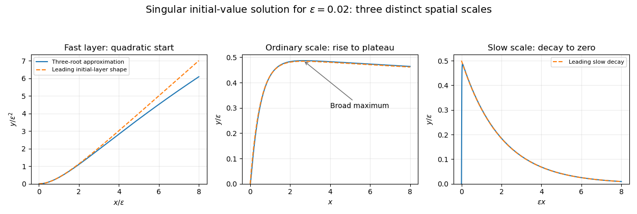
Initial quadratic rise, ordinary-scale plateau and slow decay of the singularly perturbed initial-value solution
. The sign of the parameter matters on an infinite interval. If is allowed, the singular mode grows rather than decays. For each fixed , its dominant contribution is . The extra in that exponent is needed for relative leading accuracy at fixed . The positive-parameter uniform absolute bound and decaying sketch do not extend to that regime.
Apply the stationary phase method to the real part of the exponential integral for the Bessel function of the first kind. With fixed, use oscillatory phase and oscillatory integral amplitude . The unique stationary point is , with second derivative . Its contribution isThe leading endpoint terms of the exponential integral are imaginary and do not contribute to its real part. Hence the large-argument asymptotic expansion of the Bessel function of the first kind isThis is an additive asymptotic formula: a relative ratio is inappropriate at zeros of the leading cosine. The envelope decreases like while the oscillation frequency approaches one.
Initially suppose , the usual oscillatory range. The oscillatory phase is with . Its stationary point is , since . At that pointThe stationary phase method therefore gives the Debye Bessel asymptoticThe error is additive for fixed positive bounded away from ; this formula is not uniform as , when the stationary point joins the endpoint and its curvature vanishes.
The printed condition alone includes other trigonometric branches. All defined fixed real cases can be covered as follows. If , put . Use the displayed formula with instead of , and multiply it by if , or by if . This follows from the integer-order parity , which is also obtained from the defining integral by . If , the argument is and the turning-point answer below applies, with the same parity factor. If , the stated argument is undefined.
The Bessel turning-point asymptotic comes from a cubic stationary endpoint, not an ordinary quadratic stationary point. Near ,Thus the contributing width is . On writing , the leading integral isThe oscillatory integral is understood with a vanishing damping factor. Substitution and the Gamma function Fourier integral giveThereforeThe equality uses the Gamma reflection formula. Contributions away from the degenerate endpoint are smaller. The scale explains why the preceding formula cannot be extended directly to zero angle.
Articles by others on the same topic
There are currently no matching articles.