The small root and the root near are regular perturbation roots: they stay finite as the parameter vanishes. Substitution of power series givesFor the third root, dominant balance for algebraic roots requires . The largest terms give , and the missing branch is . The sum of the three roots then yieldsThus the leading roots are , , and ; only the last is a divergent perturbation root. The first regular branch happens to have a zero limit, so retaining its first nonzero term is essential on the long spatial scale.
First take , the decaying half-line regime. If the three exact roots are , the exact initial value problem solution isThis follows either by solving the three initial-value equations or from the Laplace transform . The coefficient formula has sums and .
Retain the three leading roots but compute their coefficients without expanding their denominators. Set , , . A convenient composite asymptotic expansion isIt satisfies all three initial conditions exactly and retains the fast transient, the ordinary decay, and the slow decay. Its first two coefficients are and ; the fast coefficient is . Consequently the simpler bulk expression is , but that expression alone does not reproduce the initial derivative layer.
The absolute error estimate isTo see its uniformity, the slow-root error is , while its magnitude is and its coefficient is . The uniform error bound for nearby decaying exponentials therefore gives an contribution even for . The middle-root error is with coefficient , again giving . The fast-root error is with magnitude and coefficient , giving only . Coefficient errors are or smaller. This estimate concerns itself, rather than asserting the same uniform order for all derivatives or a relative error at its zero.
For the sketch, on one obtainsThus at the origin and rises smoothly after the fast layer. For it rises towards a plateau of height approximately , then decays on the much longer scale . The bulk maximum lies near and has height asymptotic to .
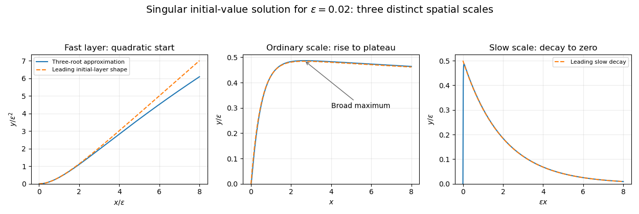
Initial quadratic rise, ordinary-scale plateau and slow decay of the singularly perturbed initial-value solution
. Details. 
The sign of the parameter matters on an infinite interval. If is allowed, the singular mode grows rather than decays. For each fixed , its dominant contribution is . The extra in that exponent is needed for relative leading accuracy at fixed . The positive-parameter uniform absolute bound and decaying sketch do not extend to that regime.
Apply the stationary phase method to the real part of the exponential integral for the Bessel function of the first kind. With fixed, use oscillatory phase and oscillatory integral amplitude . The unique stationary point is , with second derivative . Its contribution isThe leading endpoint terms of the exponential integral are imaginary and do not contribute to its real part. Hence the large-argument asymptotic expansion of the Bessel function of the first kind isThis is an additive asymptotic formula: a relative ratio is inappropriate at zeros of the leading cosine. The envelope decreases like while the oscillation frequency approaches one.
Initially suppose , the usual oscillatory range. The oscillatory phase is with . Its stationary point is , since . At that pointThe stationary phase method therefore gives the Debye Bessel asymptoticThe error is additive for fixed positive bounded away from ; this formula is not uniform as , when the stationary point joins the endpoint and its curvature vanishes.
The printed condition alone includes other trigonometric branches. All defined fixed real cases can be covered as follows. If , put . Use the displayed formula with instead of , and multiply it by if , or by if . This follows from the integer-order parity , which is also obtained from the defining integral by . If , the argument is and the turning-point answer below applies, with the same parity factor. If , the stated argument is undefined.
The Bessel turning-point asymptotic comes from a cubic stationary endpoint, not an ordinary quadratic stationary point. Near ,Thus the contributing width is . On writing , the leading integral isThe oscillatory integral is understood with a vanishing damping factor. Substitution and the Gamma function Fourier integral giveThereforeThe equality uses the Gamma reflection formula. Contributions away from the degenerate endpoint are smaller. The scale explains why the preceding formula cannot be extended directly to zero angle.
Introduce the slow time and treat independently in the method of multiple scales. WriteAt the next order,For fixed define the period average byHere inside the averages is evaluated at the leading position and velocity . Orthogonality to both fundamental harmonics is the solvability condition in the method of multiple scales: it removes the resonant forcing that would otherwise generate a secular term. Since the squared sine and cosine averages are , the amplitude-phase equations areEquivalently and at first order. These equations describe a bounded, weakly perturbed oscillation over while the amplitude remains in a range where the expansion is ordered. At zero amplitude the oscillation phase coordinate is singular; Cartesian harmonic coefficients or an equilibrium analysis should replace it.
For conservative forcing in averaged oscillator equations, , the average determining vanishes. If , thenwhose period average is zero. Thus to this order, while a position-dependent force generally shifts the oscillation phase and frequency. The exact equation also conserves the energy , consistent with the absence of amplitude drift for bounded orbits.
For the cubic position force, . ThereforeThe leading oscillation is . For positive it is a softening cubic oscillator, obtained by weakly perturbing a harmonic oscillator. The weak-force condition is ; the constant is the leading harmonic amplitude, not a claim that the exact waveform remains sinusoidal.
For velocity-only forcing in averaged oscillator equations, , the oscillation phase average vanishes: is a periodic total derivative, using an antiderivative of . Hence to first order, although the amplitude may change.
In the cubic case, , soWith , integration givesFor positive this is cubic velocity anti-damping, not damping: the exact energy derivative is . The slow solution grows and formally diverges at . The weakly nonlinear approximation loses validity before its amplitude becomes so large that is not small; its divergence is not a controlled prediction of the exact late-time solution. If , the exact zero solution should be used separately.
Let . This is the complete elliptic integral of the first kind in parameter notation; the modulus used in some definitions is . Near the endpoint, givesUse matched asymptotic expansion with an intermediate cutoff satisfying . Away from the endpoint the leading integral iswhile the endpoint integral isAdding them removes the arbitrary cutoff and gives the logarithmic endpoint asymptotic of the complete elliptic integralThe order of the next term is therefore , rather than merely . More explicitly, if ,The logarithmic correction arises from the next terms integrated through the overlap. Its coefficient can also be found by substituting into the Gauss hypergeometric equation satisfied here, , giving , .
For fixed , set and impose the data at one at each order. The leading equation gives , hence . At the next two orders,The boundary conditions give the three-term outer expansionIts ordering fails when , locating a boundary layer of thickness at zero. Put and . The rescaled equation isIts leading equation is . Matching to the positive outer value one fixes the sign and integration constant:At the next order the bracket vanishes identically, leavingThe general solution is . In the overlap its expansion isThe outer solution re-expressed on this scale has the corresponding terms . Thus matched asymptotic expansion determines , consistently in both displayed orders, and the two-term inner expansion isThis positive branch tends continuously to zero at , with a square-root cusp. An infinite endpoint derivative is compatible with the degeneracy of the original equation's coefficient.
At fixed positive the leading outer expansion satisfies . Integrating and imposing the value at one yieldsIt diverges negatively at zero, and the neglected nonlinear shift in the derivative coefficient becomes important when . Thus the relevant logarithmically enhanced nonlinear boundary layer is larger than a plain layer. Write , andFor fixed , the leading inner equation is . Matching to the outer logarithm, for which , sets the integration constant and givesIn particular the exact equation at zero is , so
An implicit inner form also checks the matching constants. With , retain without assigning it a bounded size. The leading equation is . Inverting it gives , henceIts large- match to fixes . Taking that matched leading value at zero giveswhere is the positive real branch of the Lambert W function. Its large-argument expansion reproduces the logarithm and log-log terms above. This refinement is a matched approximation, not an exact solution of the full equation; the leading slope conclusion follows directly from the first inner scaling and the exact endpoint identity.
Keep the prescribed outer slip velocity fixed when perturbing the unsteady Prandtl equation. Cancelling the base equation and retaining terms linear in the disturbance gives the linearized unsteady Prandtl equationThe no-slip boundary condition supplies at the wall; the fixed outer velocity supplies at infinity. There is no prescribed zero normal-velocity disturbance at infinity: a finite displacement-related value is permitted.
With the frozen parallel profile , , the coefficients are invariant under translations in and . Normal modes therefore separate those variables. For the mode convention used here the equations areEliminate to obtain the Prandtl normal-mode equationwith a bounded far-field . Requiring would incorrectly eliminate the proposed outer profile. For real and real , complex conjugation of the equation and its boundary conditions replaces by . This proves the stated eigenvalue symmetry. The paired modes have the same temporal growth rate , so choosing positive wavenumber loses no real physical disturbance.
Here the prescribed parallel profile is a local frozen-coefficient model. A nontrivial arbitrary with and constant outer slip is not generally an exact steady solution of the unforced unsteady Prandtl equation; its base equation would require . The following stability calculation uses the simplifying local model stipulated for the mode analysis.
Set . Away from the critical point the dominant equation is , whose solutions are multiples of . Choosing the coefficient to be zero below and one above it satisfies the wall and tangential far-field conditions. The choice makes continuous across the joining point; also makes its first derivative continuous. Its second derivative jumps. Thus it is a valid leading outer solution away from , but viscosity must smooth the join in a critical layer in a shear flow.
Near the join, . If the layer width is , matching gives . The advection side of the mode equation scales as and scales as . Balance gives . Equivalently, the eigenvalue correction balances , so the quarter-power critical layer hasSubstitution, retaining the leading terms and cancelling their common factor, gives
At order outside the layer,A solution consistent with the chosen lower branch and the wall conditions is below the join. Above it a particular solution is ; a multiple of represents an arbitrary amplitude renormalization and may be set to zero. Matching consequently requiresThe corresponding derivatives match as , on the positive side and as zero on the negative side. The matching statements require that growing homogeneous corrections be absent.
To symmetrize these different end conditions and remove and , chooseThe polynomial is itself a solution of the transformed homogeneous equation. Direct substitution, using , givesThe derivative is third order, as required by the original mode equation. Initially the two ends are along the rotated rays with real . Continuing them to the real axis is compatible with the asymptotic end conditions: the decreasing homogeneous correction behaves exponentially as and still decreases throughout the rotation from angle to zero. Thus the supplied real-axis spectral normalization uses the same recessive conditions; a complex coordinate change should not be mistaken for a real stretching alone.
For each supplied real eigenvalue , the phase-speed correction isThe mode factor has temporal magnitude . ThereforeAmong the listed indices, gives positive growth ; give decay. Hence the frozen non-monotone flow has high-wavenumber instability of a non-monotone Prandtl layer, with arbitrarily rapid linear growth as the positive wavenumber increases. The normal-mode calculation demonstrates linear instability; it is not by itself a claim about the final nonlinear state.
Articles by others on the same topic
There are currently no matching articles.