Transform in time and use the zero interior initial conditions. The Laplace transform of a derivative formula turns the wave equation into . Its transformed endpoint conditions are and . A homogeneous solution satisfying the right condition is a multiple of ; the left condition fixes that multiple. Thus, for ,Here and the denominator has no zeros in this half-plane. The initial-boundary corner at is deliberately discontinuous: the applied step launches propagating fronts, so one should not demand a globally smooth solution across them.
Rewrite the ratio of hyperbolic sines asFor , expand the denominator by the geometric series. Part (a) inverts each delayed exponential:At each finite time only finitely many terms are nonzero, so this reflected-step solution of the wave equation is locally a finite sum. The first front travels from ; the second is its sign-reversed reflection from the fixed endpoint, with repeated round trips. At the delays coincide and cancel. At the sum telescopes to for .
An equivalent standing-wave Fourier series isIts static ramp has exactly the sine coefficients , so cancellation gives the zero initial displacement in the interior. Both representations solve the equation away from the fronts and in the distributional sense across them; the convention agrees with Fourier midpoint values.
Introduce . At the midpoint, the positive fronts arrive at and the negative fronts at . HenceThe midpoint displacement is a square wave, initially zero, with period and a phase delay . At a front, choosing gives value . The dotted vertical segments below denote jumps; they are not continuous changes through intermediate displacements.
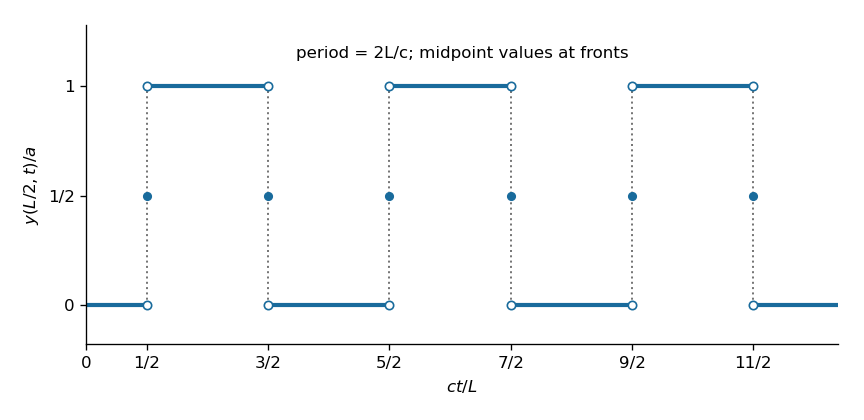
Midpoint displacement under repeated reflections of an applied step
. Articles by others on the same topic
There are currently no matching articles.