Let be the dynamic viscosity, , and the signed force exerted by sphere on the fluid. For negligible sphere inertia, this also equals the externally or internally applied force on that sphere; its hydrodynamic force is . The Stokes drag law and the axial velocity of a Stokeslet give the leading hydrodynamic mobility matrixThe factor follows from when is parallel to the line of centres. The longitudinal two-sphere mobility retains the first interaction in ; finite-size and repeated-reflection corrections are higher order.
For the linked force-free pair, . Put and . ThensoThe coefficient depends only on the current separation. For any period , , and thereforeThis is a closed integral of a single-valued function of one real shape coordinate. Since and , both spheres also have zero net displacement. Equal radii make instantaneously; unequal radii generally permit oscillatory translation, but still no mean motion. This explicit force-free two-sphere stroke is the scallop theorem: a single-parameter reciprocal deformation in a Newtonian fluid at zero inertia cannot produce net free swimming. The timing of extension and contraction cannot change that conclusion, because Stokes flow has no inertial memory.
For the externally prescribed pair, put , , andInvert the hydrodynamic mobility matrix:In a large- expansion with fixed,The isolated-drag term and the constant- interaction have zero mean. The order- term from also has zero mean, since its coefficient is constant at that order. Meanwhile,Consequently the externally driven two-sphere pump has the following phase-dependent mean force of an externally driven sphere pair:Here denotes averaging over one period. The analogous calculation gives , so at leading order, andThus the mean fluid forcing is nonzero except at or modulo . The sign changes when the phase lag is reversed. Those exceptional strokes are reciprocal: the position-space loop collapses to a line, and their mean force vanishes by reversibility, not just by this leading expansion.

An externally driven two-sphere stroke with phase lag pi over three encloses a position-space loop, and its leading mean fluid force varies as the sine of the phase lag
. Details. 
There is no contradiction with the scallop theorem. The externally imposed motion is not force-free, and the actuators prescribe two phase-shifted motions; their combined motion is not reciprocal for a generic phase. The spheres return to their prescribed positions while transferring a mean force to the fluid. This is pumping by external forcing, rather than propulsion of the freely linked one-shape-coordinate system.
The asymptotic calculation requires and persistent large separation. The minimum separation of phase-shifted sphere oscillations isThe printed condition alone does not guarantee nonoverlap or the stipulated far-separated regime. The prescribed trajectories must additionally keep this minimum well above both radii. This is a compatibility qualification on the data, not a change of the phase-dependent force calculation.
Use and in the frame translating with the sheet. At each instant, the incompressible Stokes equations areTaking their curl gives the biharmonic stream function for planar Stokes flow:in the fluid above the actual sheet. The no-slip boundary condition is imposed on material points, whose label is and whose actual horizontal position is . With ,The second sign follows from . Far above the sheet,with bounded velocity and no imposed mean pressure gradient. The positive far-field velocity arises because the sheet moves with laboratory velocity . All fields are -periodic in ; an additive function of time in is a harmless gauge. These conditions formulate the Taylor swimming sheet problem with both types of travelling deformation.
Expand and . At first order the boundary can be evaluated at :The far-field conditions are and . For a nonzero Fourier mode of wavenumber , bounded velocity selects ; the exponentially growing modes are excluded. Matching the modes and givesAn additive gauge has been set to zero. The first term is a transverse mode of a Taylor swimming sheet, and the second is a longitudinal mode of a Taylor swimming sheet. Their velocities decay at infinity. The mean first-order boundary velocity is zero, and the bounded zero Fourier mode is a constant plus a multiple of , so .
For the second-order Taylor-expanded no-slip boundary condition, the first-order displacement isThere is no explicit second-order material velocity in the prescribed motion. Hence, with all first-order derivatives evaluated at ,where and . Differentiation of the first-order solution giveson the flat reference boundary. ThereforeThe boundary conditions for the streamfunction are and . Their far-field counterparts are and .
Products of the two distinct first-order Fourier modes generate only the nonzero wavenumbers , as well as a mean. Thus the bounded general solution compatible with these data has the formThe discarded zero-mode terms would give unbounded velocity, and the discarded nonzero modes grow exponentially. The zero-mean normal velocity in periodic half-space Stokes flow is consistent with a bounded periodic flow and no far-field vertical flux. For example, integrating along the boundary yieldsThis fixes the ; the nonconstant part of fixes . All coefficients are thereby determined, but none is needed to find the mean swimming speed.
Indeed, mean boundary velocity determines Taylor-sheet swimming speed. The mean Fourier mode of is , so its horizontal velocity is the same at the boundary and infinity. Fourier orthogonality of sheet swimming modes removes the mixed product, givingHere is the average over one spatial period; a temporal average gives the same answer for these travelling waves. The laboratory swimming velocity is . The transverse wave drives motion opposite to its direction of propagation, whereas the longitudinal wave drives it in the propagation direction. Their wavenumbers enter quadratically. Thus cancels the swimming speed at order . This different-wavenumber cancellation in sheet swimming is not a claim that all higher-order swimming terms vanish.
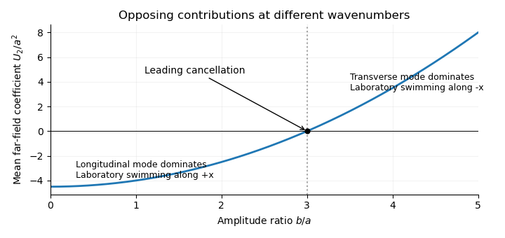
The leading sheet swimming coefficient scaled by a squared changes sign at b over a equal to three, where longitudinal and transverse contributions cancel
. Details. 
In resistive-force theory (RFT), the hydrodynamic force per unit arclength exerted by the fluid on a slender filament isHere is the unit tangent and the local velocity relative to the background fluid. The parallel and perpendicular drag coefficients of a slender filament are positive and generally satisfy ; their leading logarithmic ratio is about two. This local approximation assumes a small filament radius compared with length and curvature scales, negligible fluid inertia, and a Newtonian fluid. It represents drag by the local tangent direction and neglects nonlocal hydrodynamic interactions between separated filament segments. Boundaries, close approaches and end corrections may require slender-body theory or a more complete flow calculation. In this problem the background fluid is at rest, and the drag coefficients are taken uniform along the filament.
The rigid-body velocity in a deforming swimmer frame is the sum of translation, rotation and material deformation. With ,so, in instantaneous swimmer-frame components,The reference-frame conditions attach the origin and orientation to the filament's base and base tangent. They prevent arbitrary shape translations or tilts from being absorbed into the definition of .
The exact tangent and arclength element areSince , the local velocity is . Changing the drag tensor by its tangent correction therefore changes only at . The arclength correction is smaller still at this order. Also . Thus is sufficient at order . This assumes the small-slope expansion is uniform, .
Put and , with . The first-order local force isIts total hydrodynamic forces areTaking the moment about the swimmer-frame origin, , the second term is beyond first order. HenceFor force-free and torque-free motion, the three leading coefficients vanish. The longitudinal force immediately gives . The two transverse equations areTheir determinant is . Solving yields the first-order free swimming of a planar filament:The resistive-force theory coefficient cancels because both equations use the same transverse drag. Another interpretation is the least-squares projection of filament deformation velocity: is the best affine approximation to on . Zero transverse force and torque mean that the residual is orthogonal to and .
If is sufficiently differentiable and periodic with period , each has zero temporal mean. More explicitly,Both bracketed quantities return to their initial values over a period. Thus the first-order periodic transverse swimming velocity satisfiesThese results concern first order and swimmer-frame components. Changes of orientation can affect laboratory displacements at second order; higher-order net swimming is not ruled out.
Use the same resistive-force theory convention as before: the force density is the fluid's force on the filament. Let be the usual cylindrical azimuth. Choose the orientation of a left-handed helix so that, as increases, decreases. With , ,Reversing the orientation of the tangent leaves the local drag tensor unchanged. Define . From resistive-force theory, the relevant force-density components areThese scalar axial and azimuthal components are uniform along the helix. Integration over its contour length , and use of the axial torque density , give the axial resistance matrix of a slender helix:Thus , as also required by the Lorentz reciprocal theorem. The signs here belong to , with forces and moments on the helix. The handedness reversal of helical hydrodynamic resistance reverses but leaves unchanged. If the positive rotation direction or handedness convention is reversed, the coupling sign reverses with it.
As a check on physical admissibility, the determinant of helical resistance in resistive-force theory isTogether with , this makes the hydrodynamic resistance matrix positive definite and the viscous power loss positive. Isotropic local drag would have , so rotating a helix would not propel it in this approximation.
For the pair, use a local additive resistive-force theory model: both helices have the same drag coefficients, and inter-helix hydrodynamic interactions and unresolved end effects are omitted. The right-handed helix has resistance entries . Define the signed motor motion byThe printed relative rotation specifies a magnitude rather than which helix rotates relative to which. Choosing instead reverses all signed speeds below.
The common translation speed and zero total force and torque obeyInternal motor forces and torques cancel in these totals. IntroduceSolving the three linear equations yields the opposite-handed counterrotating helical swimmer:For , and , , so , and . The opposite-handed helices counterrotate but contribute thrust in the same axial direction. The formula satisfies the specified relative rotation without identifying either laboratory rotation rate with the motor rate.
At , the second helix supplies no hydrodynamic resistance. The remaining helix must have , and invertibility of its hydrodynamic resistance matrix forces . Formally is the rotation of a zero-resistance motor shaft or vanishing second rotor; there is no physical finite second helix to propel or to provide a reaction torque. This is the vanishing reaction rotor in a helical swimmer.
At , equal-length opposite-handed helices haveThe translation-generated axial torques cancel between the two helices, and equal counterrotation balances the rotational torques. Their propulsive forces add, rather than cancel, because handedness and rotation both reverse. These are equal-length opposite-handed helices.
For , the large reaction helix limit isThe increasingly long second helix nearly anchors the whole assembly: its very small translation and rotation suffice to balance the finite force and torque generated by the first helix. The first helix rotates at almost the full motor rate, but moving the large resistive second helix makes the common translation tend to zero. These are idealized limits of the additive local model, rather than a resolution of short-helix end effects or infinitely extended interacting filaments.
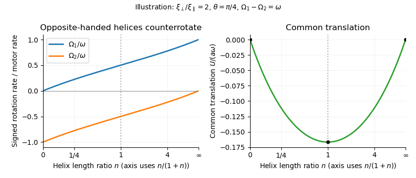
Counterrotation rates and common translation versus the right-to-left helix length ratio, showing no propulsion at zero or infinite ratio and symmetric counterrotation for equal lengths
. Details. 
Articles by others on the same topic
There are currently no matching articles.