Past exam of the mathematics course of the University of Cambridge / 2018 / iii / Paper 303 (Statistical Field Theory)

Use the usual homogeneous, local, analytic Landau-Ginzburg theory; rotational symmetry and Z2 symmetry alone do not specify locality, analyticity, or the signs of the coefficients. The local derivative expansion contains every rotational scalar with an even total number of fields:The omitted terms include all allowed higher field powers and contracted spatial derivatives. Terms differing by a total derivative are equivalent for bulk behavior with suitable boundary conditions. The displayed gradient energy assumes spatial homogeneity. If only rotations about an origin are imposed, rotationally invariant position-dependent coefficients are also possible.

In the mean-field approximation, take a spatially uniform order parameter and minimize its Landau free energy. For $\gamma >0$, $u>0$ and $r=a(T-T_c)$ with $a>0$, keeping the quadratic and quartic terms givesThe single minimum splits into two minima as the temperature passes below the critical temperature. Choosing one minimum gives spontaneous symmetry breaking of the Z2 symmetry and a continuous phase transition. The order parameter is the expectation in a selected ordered state; averaging equally over both states gives zero. A Z2 symmetry does not guarantee a continuous phase transition: a negative quartic coefficient stabilized by a positive sextic coefficient can instead give a first-order phase transition.

Relaxing the Z2 symmetry permits odd terms. A nonzero linear source generally rounds this ordinary continuous phase transition. A cubic term can instead give a first-order phase transition: for $V(\varphi )=r{\varphi }^2/2+w{\varphi }^3/3+u{\varphi }^4/4$, $u>0$ and $w\ne 0$, equal minima occur atThe order parameter jumps from zero to ${\varphi }_{\ast }$. A continuous phase transition without an exact Z2 symmetry is still possible with additional tuning; odd terms do not logically exclude it.

For the multicritical even Landau potential, set $r={\mu }^2=a(T-T_c)$ and assume an integer $n\ge 2$, ${\lambda }_n>0$ and $\gamma >0$. For $n>2$, all lower even interactions must be absent or tuned to zero to obtain these mean-field critical exponents. The stationary equation isIts nonzero solutions are minima because $V^{\prime \prime }({\varphi }_0)=-(2n-2)r>0$. Thus the order-parameter critical exponent isSubstituting into the minimum free energy density givesThe singular heat capacity per unit volume is $c_s=-T{\partial }_T^2{f}_{\min }$. Smooth variation of the other coefficients does not change the leading power. ConsequentlyFor $n=2$, this means a finite heat capacity jump, with ${\alpha }_{\mathrm{MF}}=0$; for $n=3$, the tricritical point has ${\beta }_{\mathrm{MF}}=1/4$ and ${\alpha }_{\mathrm{MF}}=1/2$. The case $n=1$ would contain only a quadratic potential and would not stabilize an ordered phase.

The Gaussian fluctuation correction near a critical point is more singular than the mean-field approximation contribution whenThis is the upper critical dimension of an even scalar interaction. Equivalently, its coupling has engineering dimension $2n-(n-1)d$, positive below $d_c$. Dominant fluctuations signal breakdown of the mean-field approximation; the Gaussian expression is not then a calculation of the exact interacting heat-capacity critical exponent. At $d=d_c$, equality of the powers allows logarithmic corrections.

Absorb $k_{B}T$ into the free energy, so the statistical weight is $e^{-F}$. Under the Gaussian fixed point rescaling, invariance of the gradient energy gives the engineering dimensionThe engineering dimensions of ${\varphi }^2,{\varphi }^4,{\varphi }^6$ are respectively $1,2,3$. Their coupling eigenvalues are $d-[{\varphi }^{2m}]$, hence $2,1,0$. The quadratic and quartic interactions are relevant operators; the sextic interaction is a marginal operator at this order.

The three steps of the momentum-shell renormalization group are:

Here $b=e^s>1$, so increasing $s$ means flowing toward longer distances. At leading order, the fast field has a Gaussian distribution with covarianceThis perturbative integration requires $k^2+{\mu }_0^2>0$ on the shell. By the Wick theorem, odd fast-field moments vanish and $⟨{\eta }^4⟩=3I_b^2$, $⟨{\eta }^6⟩=15I_b^3$. Therefore the first term of the cumulant expansion of a coarse-grained free energy isThis is the quartic interaction generated by a sextic interaction. Including the rescaling, the requested flow isIn spherical coordinates, $I_b=(2{\pi }^2{)}^{-1}{\int }_{\Lambda /b}^{\Lambda }{k}^2/(k^2+{\mu }_0^2)dk$. In particular, for ${\mu }_0^2=0$,The same integration shifts the quadratic coefficient by $90{\lambda }_0{I}_b^2$ before rescaling and adds an irrelevant constant to the free energy. Thus setting the bare quartic coupling to zero does not place the theory on the tricritical critical surface.

To calculate the sextic renormalization-group beta function to second order, let $V={\lambda }_0\int d^{3}x(\phi +\eta {)}^6$. The required cumulant expansion isThe subtraction removes disconnected contributions. The term $20{\lambda }_0{\phi }^3{\eta }^3$ at each vertex supplies the primitive sextic correction. The Wick contractions giveThe first term contains three propagators connecting the two vertices; its factor $6$ is the number of bijections between the three fields at each vertex. The second contains a local tadpole diagram at each vertex and one connecting propagator. The primitive contribution to the free energy is thereforeExpanding the slow fields about a common point gives a negative local sextic correction proportional towhere ${\chi }_b$ restricts a momentum to the shell. This connected Feynman diagram has two independent loop momenta. Other Wick contractions also generate lower interactions and tadpole diagrams; they must be included or subtracted consistently when fixing the tricritical critical surface.

To extract the logarithmic tricritical sextic beta function, use normal ordering to remove local tadpoles and tune the quadratic and quartic relevant operators. The massless three-dimensional propagator is $C(z)=1/(4\pi |z|)$. The same three-line contraction over short separations $a<|z|<ba$ givesIts positive coefficient and the negative sign of the second cumulant expansion term establish the sign of the flow. Matching this logarithm to a renormalized coupling, or performing consistent iterated shell integration, givesThe precise normalization of $C$ is not needed. In a sharp momentum cutoff scheme, simply forcing all three internal momenta into one infinitesimal shell does not extract this two-loop logarithm: the shell restrictions remove its linear-in-$ds$ phase space. The finite-shell cumulant and the logarithmic renormalized calculation above are distinct stages of the computation. Field normalization corrections at order ${\lambda }^2$ enter this renormalization-group beta function only at order ${\lambda }^3$.

A positive, stabilizing sextic coupling is marginally irrelevant in three dimensions on the tricritical critical surface. Reversing the convention for $s$ reverses the sign of the renormalization-group beta function. A negative sextic coupling without higher stabilizing powers makes the potential unbounded; moreover, the untuned bare choice $g=0$ generally flows away through its generated relevant operator.

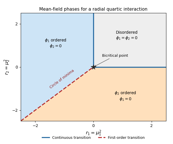
Write $r_i={\mu }_i^2$ and assume $g>0$, as required for quartic stability. In the mean-field approximation, the two-component radial quartic Landau potential isSet $x={\varphi }_1^2\ge 0$, $y={\varphi }_2^2\ge 0$. At fixed $\rho =x+y$, the quartic term is fixed and the quadratic term is minimized by assigning all of $\rho$ to the component with smaller $r_i$. Minimizing over $\rho$ then givesThe resulting phase diagram has these regions:

On $r_1=r_2=r<0$, the symmetry is enhanced to the orthogonal group $O(2)$, and the minima form the circleMixed-component minima occur on this line, rather than in an open coexistence region. Crossing the negative diagonal swaps the selected component discontinuously: this is a first-order phase transition, also called a spin-flop transition. For example, holding $r_2=r<0$ fixed and moving $r_1$ across $r$, the derivative $\partial f_{\min }/\partial r_1$ jumps from $-r/(8g)$ to zero. The angular degeneracy exactly on the line does not remove this discontinuity.

The positive half-axis $r_1=0$, $r_2>0$ is a continuous phase transition, as is $r_2=0$, $r_1>0$. Their endpoint at $(0,0)$ is a bicritical point, where the two continuous boundaries meet the first-order negative diagonal. Approaching the origin radially makes the ordered amplitude vanish continuously. The negative half-axes lie inside ordered phases and are not additional transition lines. There are two continuous half-axis boundaries and one first-order negative diagonal, meeting at the origin.

At the Gaussian fixed point, $[{\varphi }_i]=(d-2)/2$, so all three quartic couplings have engineering dimension $d-4[{\varphi }_i]=4-d$. ThusTake $A>0$ and $ϵ>0$, as in the perturbative epsilon expansion. Define $x=A{g}_1/ϵ$, $y=A{g}_2/ϵ$, $z=A\lambda /ϵ$. The renormalization-group fixed point equations becomeIf $z=0$, each of $x,y$ is independently $0$ or $1/36$, giving four renormalization-group fixed points. If $z\ne 0$, subtracting the first two equations givesThe branch $x+y=1/36$ forces $z=1/12$; inserting this in the first equation yields a repeated root $x=y=1/72$. Hence every nonzero-$z$ solution has $x=y$. Then $z=1/8-3x$, andhas roots $x=1/40$ and $x=1/72$. The complete list of six coupled Ising fixed points near four dimensions, in coordinates $(g_1,g_2,\lambda )$, isThe internal symmetries of these renormalization-group fixed points are:

The last point displays the field-rotation equivalence of decoupled Ising theories. With the orthogonal transformation ${\psi }_{\pm }=({\varphi }_1\pm {\varphi }_2)/\sqrt{2}$,It is the same pair of decoupled Ising models written in fields rotated by $45^{\circ }$, but remains a distinct coordinate solution of the stated renormalization-group beta functions. Here $D_4$ denotes the dihedral group of order eight; an alternative convention calls it $D_8$. We have described linear internal transformations preserving the gradient energy; free massless sectors also have constant scalar-field shift symmetries. At $ϵ=0$, the six coordinates coalesce at the Gaussian fixed point.

Assume $g>0$ for stability. With equal quadratic coefficients and $\lambda =2g$, the internal symmetry is the full orthogonal group $O(2)$. In two dimensions at positive temperature, with short-range interactions, the Mermin-Wagner theorem forbids spontaneous symmetry breaking of this continuous symmetry. Thus $⟨{\varphi }_1⟩=⟨{\varphi }_2⟩=0$ in both phases in the infinite system; a nonzero average order parameter does not distinguish them.

Instead measure the correlation functionThe low-temperature phase has quasi-long-range order and algebraic correlations; the high-temperature phase has a finite correlation length and exponential correlations. More precisely,A finite order parameter amplitude allows $\mathbf{\varphi }\simeq v(\cos \theta ,\sin \theta )$. Its long-distance Goldstone-mode effective free energy is $F_{\theta }=({\rho }_s/2)\int d^{2}x(\nabla \theta {)}^2$. Restoring the Boltzmann constant and using the renormalized phase stiffness, the thermal phase fluctuations giveThe Berezinskii–Kosterlitz–Thouless transition separates vortex-antivortex binding from unbound vortex defects. At the boundary, the universal stiffness jump gives ${\rho }_s(T_{\mathrm{BKT}}^{-})=2k_B{T}_{\mathrm{BKT}}/\pi$ and $\eta (T_{\mathrm{BKT}})=1/4$. The low-temperature phase stiffness is nonzero; it vanishes at long distances in the disordered phase. The exact transition location is fluctuation dependent and cannot be obtained just by setting the bare ${\mu }^2$ to zero.