Use the Cartesian streamfunction convention , . Taking the curl of the incompressible Stokes equation eliminates pressure and gives the biharmonic stream function for planar Stokes flow equationThe material points have no horizontal velocity in the swimming frame and have vertical velocity . The no-slip boundary condition is thereforeAt infinity the laboratory fluid is at rest, so in this translating frame it moves with :Velocity and its perturbations are periodic in , with period , and the pressure has no imposed mean gradient. The Taylor swimming sheet is force-free; the unbounded problem's bounded far-field velocity enforces the absence of mean shear. An additive constant in the streamfunction has no physical effect.
Expand and . A Taylor expansion of the sheet boundary conditions about givesThe first-order Fourier mode is , with , , and . Decay excludes the growing exponentials, leaving . The two boundary values give :There is no first-order mean boundary motion. Boundedness excludes mean shear, so .
At second order the Taylor-expanded no-slip boundary condition iswith , , and at infinity. Set the irrelevant boundary constant to zero. The general relevant solution contains a zero Fourier mode and a second harmonic:Bounded velocity eliminates and growing harmonics. Averaging the tangential boundary condition gives . This is the mean boundary velocity determines Taylor-sheet swimming speed principle: the remaining mean velocity is uniform and equals the far-field velocity. ThereforeThe absence of odd powers follows because changing the amplitude sign is just a half-wavelength translation. Although unnecessary for the speed, the oscillatory solution can also be written explicitly as .
The wall is stationary in the laboratory and moves with velocity in the sheet frame. Its no-slip boundary condition is thereforeThe first equation prescribes wall tangential velocity; the second imposes zero normal velocity. The streamfunction may have a constant mean value on the wall, set by the fluid transport, and that constant need not equal its value at the sheet.
The wall removes the far-field decay condition and instead imposes , . The force-free condition eliminates any first-order mean shear; since mean sheet tangential velocity is zero, . Thus , whereStart with the hyperbolic function form . The lower conditions give , . Defining , the wall conditions giveConsequently the first-order flow for Taylor-sheet swimming next to a rigid wall isFor , ensures a nonzero denominator; as , this reduces to the unbounded first-order field on every fixed height interval.
At the sheet, the second-order conditions are and . At the wall, and . The general solution has a polynomial mean mode and a second harmonic with exponentials , as in the unbounded calculation.
Let . The averaged Stokes equation, with periodic pressure and no imposed mean pressure gradient, gives . The total horizontal hydrodynamic force on the sheet is opposite to the mean shear force on the flat wall. Since the swimmer is force-free, , making the mean velocity constant. Matching its values at the sheet and wall therefore givesThe previous part gives , henceThis determines the speed without solving the second-harmonic flow. The force constraint matters: prescribing a translating sheet without imposing zero net force would allow a mean shear and would not determine a unique swimming speed.
Since , the speed enhancement isThe strict inequality follows from . It tends to one as the wall recedes, while gives in a narrow gap. The wall enhances the mean pumping generated by transverse boundary motion. This small-amplitude limit requires ; letting the wall collide with a wave crest falls outside the expansion.
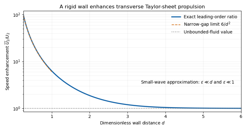
Wall enhancement of transverse-sheet swimming
. The leading swimming-speed ratio is greater than one for every finite gap and approaches one for a distant wall. The narrow-gap divergence is used only while the wave amplitude remains much smaller than the gap. Details.
The first term is the local viscous force per unit length from resistive-force theory. With unit tangent vector , the drag tensor gives , where is velocity relative to the fluid.
The second term is the bending force of an inextensible filament. Varying its energy gives bulk force density . The final term, , is the force density from filament tension; is the Lagrange multiplier enforcing . At low Reynolds number, these forces balance without a filament acceleration term.
With mass, length, and time dimensions , the coefficients haveThus the drag coefficients have the dimensions of dynamic viscosity, the filament bending modulus has dimensions force times length squared, and tension has dimensions force.
In the small-slope Monge representation, , , and the leading transverse velocity is . With no imposed axial prestress, the induced filament tension is second order in transverse amplitude, so its transverse contribution is higher order. The transverse component of force balance reduces to the small-slope elastohydrodynamic filament equationAn externally imposed zeroth-order tension would instead add .
For the transverse motion, the off-diagonal part of the resistive-force theory tensor gives axial propulsive force density to second order. Its integral isSubstitute the bending equation and integrate by parts:The boundary expression for transverse filament thrust is thereforeOnly endpoint slope, bending moment, and shear enter this expression. Exact inextensibility also generates second-order longitudinal material motion; if that motion is retained in instantaneous total axial drag, it adds . For a periodic deformation with fixed axial base position, that additional term has zero cycle average. Thus the displayed formula is the transverse propulsive contribution and also gives the cycle-averaged propulsive force.
A periodic displacement with angular frequency has . Balancing this viscous forcing with bending over length gives . Thus the elastohydrodynamic penetration length and sperm number areSince , the fourth root has dimensions length, as required.
With , , and , the bending equation becomesThe defining balance cancels both coefficients, giving . A large sperm number means that the periodically forced response decays before reaching the distant end.
For the long filament, take the time-periodic solution of the dimensionless bending equation, after transients have decayed. Write . Then , so the spatial exponents satisfy . Define and . The two roots with negative real part are and ; the other roots violate decay at infinity.
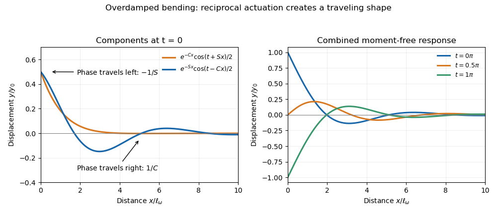
Hence . The driven displacement gives , while the zero bending moment gives . Since , . The oscillatory bending of a moment-free semi-infinite filament isHolding each wave phase constant gives its dimensionless phase velocity:The first travels toward the actuator and attenuates over length ; the second travels away and attenuates over the longer length . These are spatially damped phase patterns in an overdamped bending equation, not two undamped inertial beam waves. Their combination satisfies both displacement and zero-moment conditions at the driven end.

Articles by others on the same topic
There are currently no matching articles.