Past exam of the mathematics course of the University of Cambridge / 2024 / iii / Paper 316 (Planetary System Dynamics)

Put the star at the origin, take $\hat{\mathbf{z}}$ along the line of sight toward the observer, and let $\hat{\mathbf{x}}$ point North in the plane of the sky. The $\hat{\mathbf{y}}$ direction is then $90^{\circ }$ anticlockwise from North. Draw the ascending node on the sky plane at position angle $\Omega$, tilt the circular Kepler orbit through the orbital inclination $I$ about that nodal line, and place the planet an angle $f$ along the orbit from the ascending node. The direction of increasing $f$ must cross the sky plane toward $+\hat{\mathbf{z}}$ at $f=0$.

A convenient orthonormal basis in the orbital plane isHere ${\mathbf{e}}_1$ points along the nodal line and ${\mathbf{e}}_2$ fixes the required sense of motion. The planet lies at $\mathbf{r}=a(\cos f{\mathbf{e}}_1+\sin f{\mathbf{e}}_2)$; this relation also specifies all the labels required in the sketch.

Resolving $\mathbf{r}=a(\cos f{\mathbf{e}}_1+\sin f{\mathbf{e}}_2)$ into the sky coordinates givesIn particular, $z=0$ at the orbital nodes, and $dz/df=a\sin I>0$ at $f=0$, so that node is indeed the ascending node.

The projected separation isRotating the projected coordinates through $-\Omega$ gives components $a\cos f$ along the nodal line and $a\cos I\sin f$ perpendicular to it. The position angle is therefore most safely written with the quadrant-preserving functionor, wherever the corresponding tangent is finite,

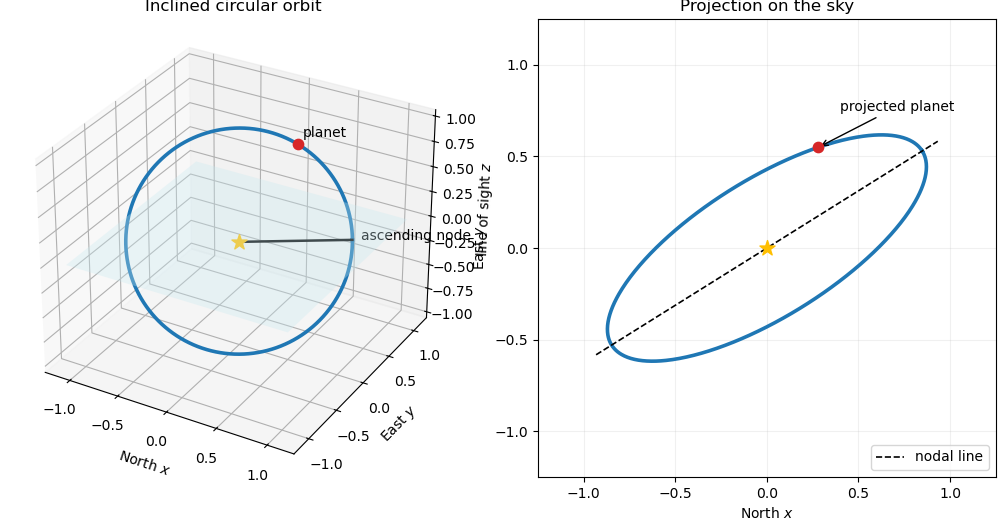
For the nearly edge-on orbit $I=\pi /2-I^{\prime }$ with $I^{\prime }\ll 1$, the small-angle approximation gives $\cos I=\sin I^{\prime }=I^{\prime }+O(I^{\prime 3})$. HenceAlso,Thus, on a branch where $\cos f>0$ and with separation measured in units of $a$,as stated. The absolute value is required when $R_{\mathrm{sky}}$ denotes the nonnegative separation over the whole orbit.

The oriented normal vectors to the planet and dust-belt planes areTheir inner product is the cosine of the mutual inclination, soIf ${\varphi }_d=\Omega$, this reduces to $\cos I_m=\cos (I-I_d)$; equal inclinations then give $I_m=0$. If both planes are face-on, it likewise gives $I_m=0$, independently of their undefined nodal longitudes. Reversing an observationally unidentified ascending node by $\pi$ produces the familiar orbital-plane orientation degeneracy for an axisymmetric belt.

Let $\Delta =\Omega -{\varphi }_d$. From part (iii), $\varphi -{\varphi }_d=\Delta +(\varphi -\Omega )$ and $\tan (\varphi -\Omega )=\cos I\tan f$. The tangent addition formula therefore givesor, without singular coordinate tangents,For $I=\pi /2-I^{\prime }$ with $I^{\prime }\ll 1$, smooth choice of the angular branch gives

Coplanarity requires both $I=I_d$ and $\Omega ={\varphi }_d$, up to the orbital-plane orientation degeneracy. Under that hypothesis the measured planet angle must obeyFor a nearly edge-on belt this offset is small except close to the projected crossings where $\cos f=0$. Measurements at several orbital phases can therefore test the entire projected ellipse: a systematic offset from the predicted relation implies a nonzero mutual inclination. A single projected location generally cannot establish coplanarity because $f$, the front-back branch, and the nodal orientation can be degenerate.

An exterior misaligned planet exerts an orbit-averaged secular torque on each belt orbit. In the hierarchical limit $a_d\ll a$, its leading quadrupole approximation drives nodal precession about the planet's orbital angular-momentum axis at a rate of orderup to a coefficient of order unity. Because this rate varies across a radially extended belt, differential nodal precession winds an initially flat belt into a warp and eventually a vertically thick, phase-mixed structure. Collisions can damp the free inclinations and make material approach a forced or Laplace plane; at sufficiently large mutual inclination, coupled eccentricity-inclination evolution such as the Kozai–Lidov mechanism may also become important.

Write the distributed fragment power-law size distribution as $n(D_f)=K_f{D}_f^{-{\alpha }_f}$. A spherical fragment has mass $\pi \rho D_f^3/6$. Since this population contains one half of the target mass,and henceThe distributed fragments have total geometric cross-sectionThe single fragment containing the other half of the mass has diameter $2^{-1/3}{D}_t$ and cross-section $\pi D_t^2/(42^{2/3})$. Therefore the exact result within the model isFor $D_{\max ,f}\gg D_{\min ,f}$ and $3<{\alpha }_f<4$, area is dominated by the smallest distributed fragments while mass is dominated by the largest, so normally the first term is negligible and

The half-target mass assigned to equal fragments containsfragments. Their total geometric cross-section is consequentlyIgnoring the negligible single largest fragment in ${\sigma }_{\mathrm{tot},1}$,For example, if $D_f=D_{\min ,f}$, this ratio is $({\alpha }_f-3)(D_{\max ,f}/D_{\min ,f}{)}^{4-{\alpha }_f}/(4-{\alpha }_f)$ and is large for a broad size range. This reflects the inverse-size cross-section per unit mass of equal-density spherical fragments: concentrating the mass at small $D_f$ creates more area.

Let the belt contain $n(D)dD=C{D}^{-\alpha }dD$ bodies. Its total mass fixesFor equal mass density, an impactor of diameter $D$ supplies specific impact energyThus catastrophic disruption requires $D\ge D_{\mathrm{cc}}=X_c{D}_t$, whereThe impactor number density per diameter is $C{D}^{-\alpha }/V$. Neglecting gravitational focusing, the geometric collision cross-section is $\pi (D_t+D{)}^2/4$, so the exact catastrophic planetesimal collision rate in this model isEquivalently, with $A=\pi C{v}_{\mathrm{rel}}/(4V)$,If $D_{\min }\ll X_c{D}_t\ll D_t\ll D_{\max }$, the steep distribution makes impactors just above $X_c{D}_t$ dominate and their collision cross-section is approximately $\pi D_t^2/4$. HenceThis approximation also assumes a common $v_{\mathrm{rel}}$ and size-independent catastrophic disruption threshold $Q_D^{\ast }$.

A collision producing cross-section $\sigma$ has target diameterby part (ii). The production rate of clumps above ${\sigma }_{\mathrm{tot}}$ is the number of targets in each size interval times their per-target catastrophic rate. Therefore, with $D_0=\max (D_{\min },D_{{\sigma }_{\mathrm{tot}}})$,Using the small-impactor approximation from part (iii) givesWhen $D_{\min }\ll D_{{\sigma }_{\mathrm{tot}}}\ll D_{\max }$, this reduces toAssigning each event to its much larger target avoids double-counting collisions in this $X_c\ll 1$ approximation.

For the Dohnanyi collisional cascade exponent $\alpha =7/2$ and $D_{\max }\gg D_{\min }$,Substitution in part (iv) yieldsThusThe $M^2/V$ dependence is the pair-collision scaling. Longer-lived clumps are more numerous, stronger bodies disrupt less often, and smaller fragments put more geometric cross-section into each event. At fixed total mass, increasing $D_{\max }$ lowers the normalization of the power-law size distribution and therefore lowers the event rate.

The impact gives fragments a spread of orbital energy and specific angular momentum. Their resulting spread of mean motion lets Keplerian shear stretch a compact dust clump into an arc and then a ring, while the spread of orbital frequencies causes phase mixing. Size-dependent radiation-pressure coefficients immediately place small grains on different eccentric or even radiation-pressure blowout orbits; Poynting–Robertson drag and stellar-wind drag then alter their orbits on longer timescales. Further collisions grind or disperse the clump, and planetary perturbations can accelerate mixing.

These processes depend strongly on $D_f$. Small grains have larger radiation-force-to-gravity ratios and generally shorter collisional or drag lifetimes, while larger fragments remain closer to the parent orbit but can preserve a velocity-dispersion-driven clump for longer. The lifetime also depends on collision location, ejection velocities, optical depth, and orbital radius. A universal fixed $\Delta t$ is therefore a useful population-model approximation, not a literal property of every collision; a size- and event-dependent lifetime distribution is more realistic.

Since the binary separation and mean motion are both one, the Kepler third law givesThe center of mass condition puts the bodies atin the rotating reference frame. Thus the sketch has $M_1$, $O$, and $M_2$ in that order along the $x$ axis, with $P=(x,y)$, andIn the inertial sketch this entire configuration rotates uniformly about $O$.

At a Lagrange point, the test particle is stationary in the rotating reference frame, so $F=G=0$. On the $x$ axis, $y=0$ makes $G=0$ automatically. The singularities at the two masses split the axis into three intervals, and the balance between gravity and centrifugal acceleration gives one root of $F=0$ in each interval. These are the three Collinear Lagrange points $L_1,L_2,L_3$.

For an off-axis equilibrium, $y\ne 0$. Put $A_i=1-r_i^{-3}$. ThenwhileHence $A_1=A_2=0$ and therefore $r_1=r_2=1$. The two intersections of unit circles centered at $M_1$ and $M_2$ form equilateral triangles with the binary, giving the Triangular Lagrange pointsTogether with the three collinear points, these are the five equilibria of the circular restricted three-body problem.

At $L_3$, the ordering is $L_3,M_1,O,M_2$. Since $r_1=1+\beta$,The equation $F=0$ becomesWriting $ϵ={\mu }_2/{\mu }_1\ll 1$ and retaining first order in $\beta$ and $ϵ$ givesConsequentlyThe negative sign says that $L_3$ is slightly less than one binary separation from the dominant mass $M_1$.

The required Taylor series giveSeek $\beta =aϵ+b{ϵ}^2+O({ϵ}^3)$. Substitution in the exact equation from part (iii) gives successivelyThus $a=-7/12$ and $b=7/12$, so

Let $X=x-x_{L_3}$ and $Y=y$ be the displacement from the L3 Lagrange point, and put $U=\dot{X}$, $W=\dot{Y}$. The first-order linearization of a dynamical system iswhere every derivative is evaluated at $L_3$. For the state vector $\mathbf{\xi }=(X,Y,U,W{)}^{\mathsf{T}}$, this becomesThe question's reuse of $\mathbf{X}$ for the state vector is only notation; its first two entries are the small displacements $X,Y$, not the absolute coordinates.

Write $d_1=x+{\mu }_2$ and $d_2=x-{\mu }_1$, so $r_i^2=d_i^2+y^2$. Sincedirect differentiation givesEvery Collinear Lagrange point has $y=0$, and in particular

At the exterior $(p+q):p$ mean-motion resonance,Using the Kepler third law for $M_{\ast }\gg M_1$ givesThe disturbing function is a Fourier series in integer combinations of the orbital angles. The D'Alembert characteristic permits the eccentric termAway from resonance, terms with rapidly circulating angles average away. Here, however,so ${\varphi }_1$ is a slow resonant argument. Successive astronomical conjunctions then act coherently, making this term dominate the long-period resonant dynamics even though a $q$th-order resonance has coefficient proportional to $e^q$ at small eccentricity.

At periapsis, $\lambda =\varpi$. If the planet has longitude ${\lambda }_0$ there, thenso ${\varphi }_1/p$ is the angular displacement of periapsis from the planet, modulo $2\pi /p$. At an astronomical conjunction, $\lambda ={\lambda }_1={\lambda }_c$, andso ${\varphi }_1/q$ is the conjunction longitude measured from periapsis, with the $q$ possible branches differing by $2\pi /q$.

The planet's mean motion is $n_1=(p+q)n/p$. Hence the synodic period, or mean interval between conjunctions, iswhere $T=2\pi /n$ is the planetesimal's orbital period.

For the 8:5 resonance, $p=5$ and $q=3$. Five planetesimal periods equal eight planetary periods, so the curve closes afterStarting at conjunction at apoapsis gives ${\varphi }_1=q\pi =3\pi \equiv \pi (\mathrm{mod}2\pi )$. In the frame rotating with the planet, let $\theta$ be the planetesimal's longitude relative to the fixed planet. At periapsis, $5\theta ={\varphi }_1$ modulo $2\pi$, so the five possible periapsis directions areAt apoapsis, ${\varphi }_1=5\theta +3\pi$, givingA sketch should therefore show a five-lobed rotating-frame rosette centered on the star, with the fixed planet on the $\theta =0$ ray, five outer turning points separated by $72^{\circ }$, and five inner turning points halfway between their rays. Successive orbits visit these points in resonance order before the fifth orbit closes the pattern.

If an exterior planetesimal reaches conjunction just before apoapsis, its radius is increasing. The closer pre-conjunction pull from the trailing inner planet removes more specific angular momentum than the more distant post-conjunction pull restores. Its semi-major axis falls, its mean motion rises, and the next conjunction moves later in its orbit toward apoapsis. A conjunction just after apoapsis produces the reverse imbalance: the stronger post-conjunction pull adds angular momentum, raises the semi-major axis, and shifts the next conjunction earlier. The conjunction phase is therefore restored toward apoapsis.

The symmetric configuration has one of the three conjunction branches at apoapsis and the other two symmetrically placed. It hasso the resonant argument librates about $180^{\circ }$.

At conjunction, the planetesimal's mean anomaly isIf ${\varphi }_1=\pi +\delta$ with $|\delta |\le \Delta {\varphi }_1\le \pi$, the conjunction branch that can come closest to periapsis hasLet $E_{min}$ solve Kepler's equationAt that phase the orbital radius is $r_{min,c}=a(1-e\cos E_{min})$. A geometrical close encounter is possible only ifwhere $R_{\mathrm{enc}}$ may be chosen as the planet's Hill radius or another encounter distance. With a point planet, set $R_{\mathrm{enc}}=0$. This implicit inequality is the requested eccentricity constraint as a function of $\Delta {\varphi }_1$.

The weaker necessary condition that the orbits cross isIt becomes sufficient for phase access only as $\Delta {\varphi }_1\to \pi$, when a conjunction can approach periapsis. Smaller libration amplitude keeps conjunctions farther from periapsis and requires a larger eccentricity than this orbit-crossing bound.

For each point $(\Delta {\varphi }_1,e)$, sample $\delta \in [-\Delta {\varphi }_1,\Delta {\varphi }_1]$ and the three conjunction branchesFor every branch, solve Kepler's equation for the eccentric anomaly, evaluate $r=a(1-e\cos E)$, and minimize the planet-planetesimal separation over $\delta$ and $k$. Mark the point as encounter-capable when this minimum is below a chosen $R_{\mathrm{enc}}$, naturally the Hill radius for strong scattering. Repeating this calculation on a grid traces the boundary in the $\Delta {\varphi }_1$--$e$ plane.

Direct integrations of the circular restricted three-body problem can then refine the geometric map by allowing the resonant argument, eccentricity, and conjunction kicks to evolve self-consistently. The integrations distinguish merely orbit-crossing initial data from trajectories that actually enter the encounter region, and reveal chaotic layers near the boundary.