Past exam of the mathematics course of the year 1 of the natural sciences course of the University of Cambridge / 2017 / Paper 1 / 14

An interior stationary point has vanishing gradient:For a differentiable function, this is the necessary first-order condition for an interior local minimum or local maximum.

Write $A=f_{xx}$, $B=f_{xy}$, $C=f_{yy}$ at the stationary point, and let $D=AC-B^2\ne 0$. Under the usual second-order Taylor expansion hypothesis, the second-derivative test givesIndeed the quadratic term is $(A{\xi }^2+2B\xi \eta +C{\eta }^2)/2$. For $A\ne 0$, completing its square gives $[A(\xi +B\eta /A{)}^2+(D/A){\eta }^2]/2$. The two coefficients have the same positive sign, the same negative sign, or opposite signs in the respective cases. A negative $D$ also forces the two Hessian eigenvalues to have opposite signs, including the case $A=0$.

There is a qualification to the printed assumptions: existence of second partial derivatives only at the point does not ensure the needed quadratic approximation. Continuous second partial derivatives in a neighborhood are sufficient. The existence of second partial derivatives does not justify the Hessian test: for example, the function $g=x^2+y^2-6x^2{y}^2/(x^2+y^2)$ away from the origin, extended by $g(0,0)=0$, has Hessian $2I$ at the origin but $g(t,t)=-t^2$ and $g(t,0)=t^2$. Thus the classification above uses the standard additional regularity assumption, which the smooth function in part (b) satisfies.

Put $G=(x^2+y^2)/2+a{x}^4/4$, so $f=e^G>0$. Since $f_x=f{G}_x$ and $f_y=f{G}_y$, its stationary points satisfyThe origin occurs for every real $a$. There are two additional points only for $a<0$, at $x=\pm 1/\sqrt{-a}$.

At a stationary point, the Hessian matrix simplifies because $\nabla G=0$:At the origin this is $I$, so $(0,0)$ is a strict local minimum for every $a$, with $f=1$. If $a\ge 0$ it is also the unique global minimum, since $G\ge 0$ with equality only there. For $a<0$, the two extra points have $1+3a{x}^2=-2$, so their Hessian has opposite-sign eigenvalues. ThusThere are no local maxima. When $a<0$, the origin is not a global minimum: $f(x,0)\to 0$ as $|x|\to \infty$, but $f$ never attains zero.

Because the exponential function is strictly increasing, the level sets $f=L>0$ are exactly those of $G=\ln L$. For $a=1$ they satisfyThere are no contours for $L<1$, the level $L=1$ is the origin, and $L>1$ gives nested closed ovals symmetric about both axes. Their stronger fourth-power growth in $x$ makes them relatively narrower horizontally as the level rises.

For $a=-1$, the contour equation becomesThe central local minimum is surrounded by closed ovals for $1<L<e^{1/4}$, accompanied by outer open branches. At $L=e^{1/4}$, the level passes through the two saddle points $(\pm 1,0)$ and changes its connectivity. Levels $L<1$ have only outer branches, while levels above the saddle value have an upper and a lower branch. The sketch is restricted to the requested square; labels give $G=\ln f$, so they identify the corresponding contours of $f$ without exponentially large labels.

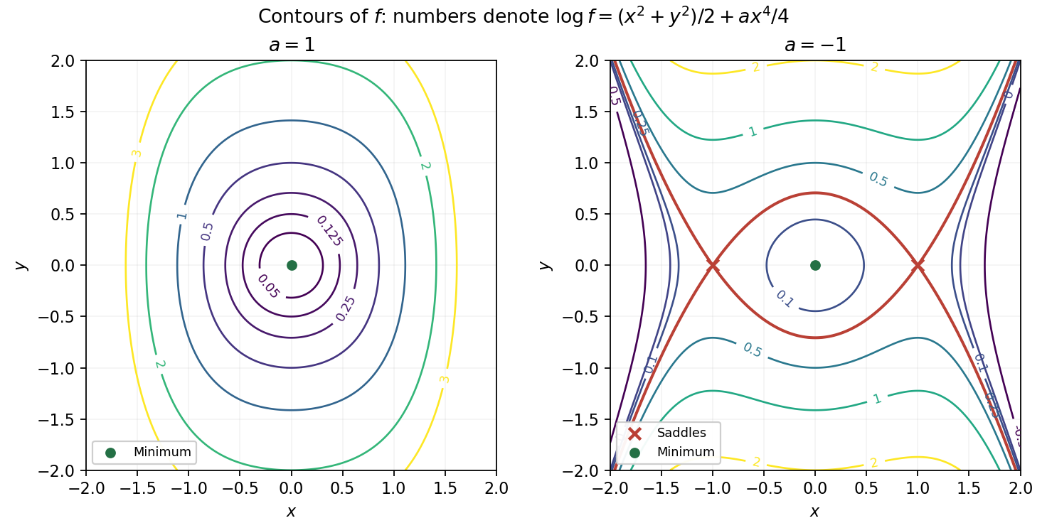
For $a=-1$, the local minimum at the origin has $f=1$. Its full level set isThe connected component containing the minimum is just the isolated origin. The same level also has the outer branches $y=\pm \sqrt{x^4/2-x^2}$ for $|x|\ge \sqrt{2}$; these are different connected components, not curves approaching the origin.

Both saddle points $(\pm 1,0)$ have $f=e^{1/4}$. Their common level set factors asIts explicit equations are thereforeThe two parabolas cross at each saddle, explaining the change of contour connectivity there. Each displayed equation can be restricted to the square of part (ii) if only that sketch window is wanted.