On the negative half-line, an antiderivative of is . The fundamental theorem of calculus therefore givesThe negative sign agrees with the negative integrand throughout the interval.
The double-angle trigonometric identity makes the integrand . The integration by substitution , , gives
Differentiate each coordinate with respect to the parameter and use the chain rule:Both coordinates are defined where and . As a check, there, so the same derivative is .
Writing the polynomial as , direct evaluation gives and . A polynomial is continuous, so the intermediate value theorem guarantees a polynomial root between them. Trying the integer gives , hence is a root.
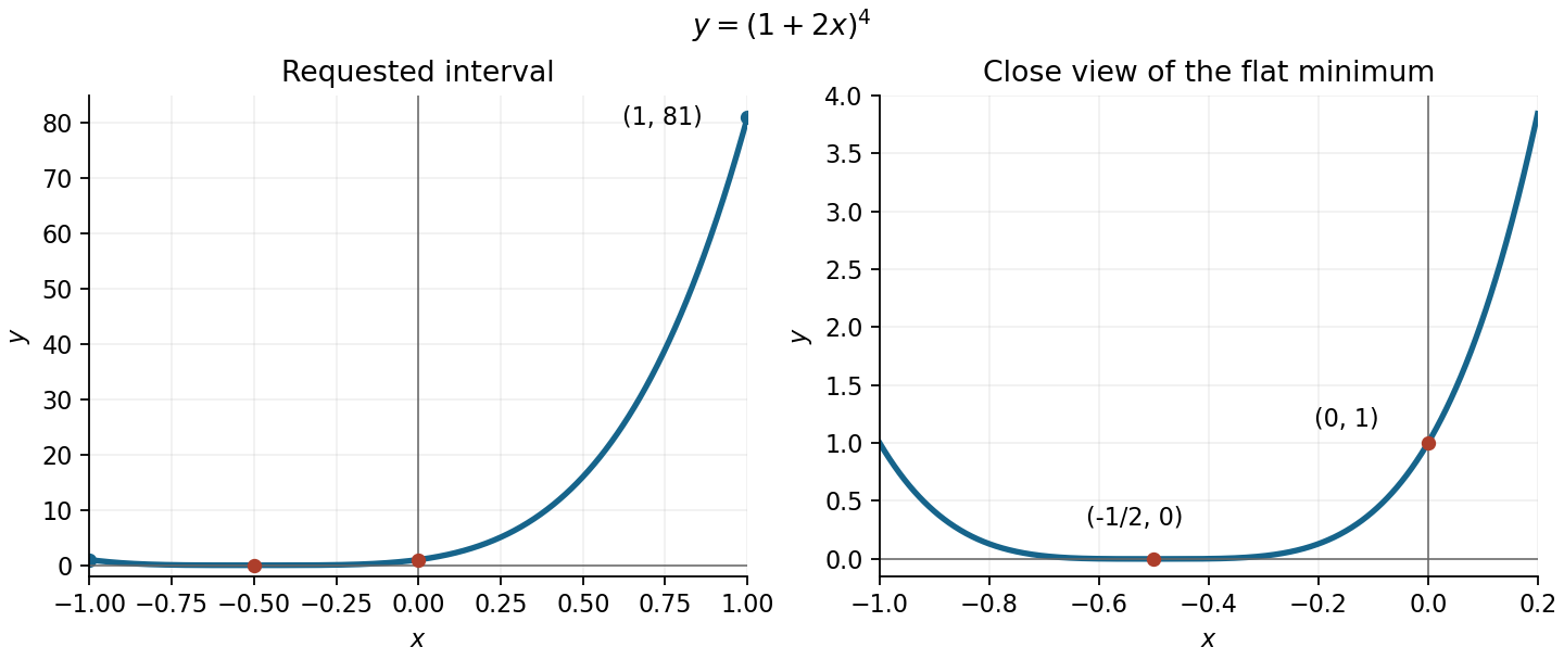
The function graph is a horizontally shifted and scaled fourth power. It is nonnegative and touches the horizontal axis at its fourfold polynomial root. The axis intersections areThe derivative is , so the graph decreases to its flat local minimum at and then increases. Its endpoint values on the requested interval are and . The original sketch includes a closer view of the minimum so that the small values are visible beside the much larger right endpoint.
Put . The double-angle trigonometric identities imply . Since is in the first quadrant, the positive square root is required. The half-angle identities then give the requested expression in terms of :
The double-angle trigonometric identity gives , or . Preserve both factors: contributes the endpoint, while contributes the interior solution. In the specified interval,
For , the separable differential equation gives . Integrating gives , orEach solution is considered on an interval not containing its pole. The additional stationary solution is excluded by the stated condition.
The initial condition gives , hence . ThusThe displayed interval is the maximal connected interval containing the initial point ; the solution of a differential equation diverges at .
In polar coordinates, , , with . Thus the polar form of a complex number isHere is its complex modulus; for , the complex argument is determined modulo . At the angle is undefined, although every value of gives the same point when .
For , the complex logarithm is , where . ConsequentlyA specified branch chooses one continuous determination of the complex argument on an appropriate cut domain. For the usual principal-value convention use the principal argument . A formula using only would lose the quadrant information; it is a valid local angle only with the appropriate additive multiple of .
Expand the defining complex exponential functions:Thus the real part and imaginary part of the hyperbolic cosine are
A constant real part means , so its level sets are the concentric circlesTheir radii are strictly positive. The real part is independent of the logarithm's branch, so there is no branch ambiguity in these circles.
For , the equation is . If , complete the square to obtainThese circles have centres on the real axis and are tangent to the imaginary axis at the excluded origin. Positive puts the circle to the right, negative to the left. The separate case gives the punctured imaginary axis . The sketch uses an open marker at the origin to emphasize that is never defined there.
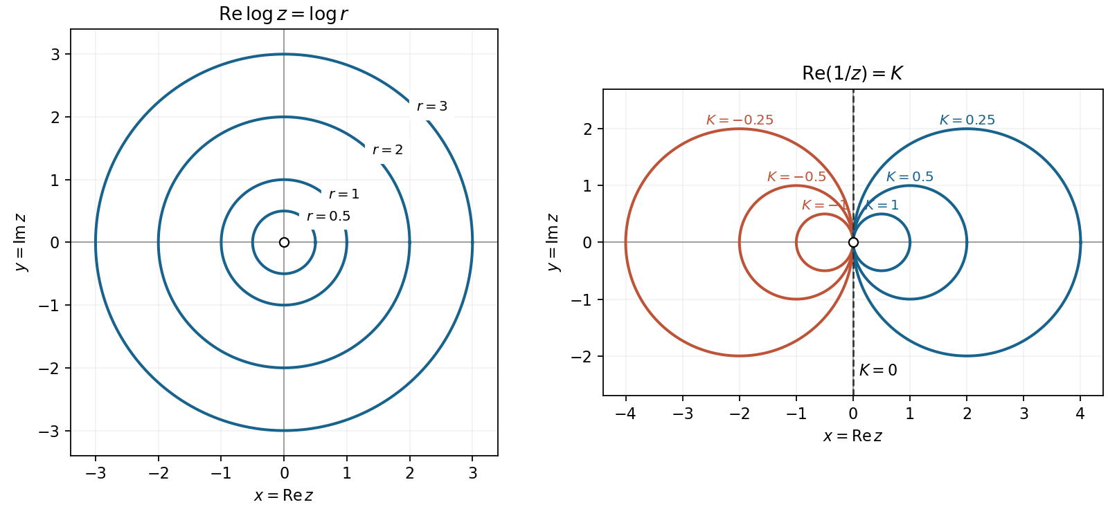
Constant real-part contours of the complex logarithm and reciprocal
. Details. Set . The hyperbolic cosine equation becomes , hence . Its two polynomial roots are , both negative. Taking every value of the complex logarithm yieldsSince , their real logarithms have opposite signs. All solutions are thereforeThe positive real constant is also , the inverse hyperbolic cosine of . Substitution gives for both signs and every integer .
Assume is continuously differentiable near the point of interest on , and that the relevant denominators below are nonzero. The total differential on the surface isHolding fixed gives , so the implicit function theorem givesWhen , their product proves the reciprocity rule for constrained partial derivatives:Similarly, holding or fixed gives and . With , multiply the three ratios:This is the cyclic partial derivative identity. Nonzero denominators and local differentiable coordinate representations are substantive assumptions: at a singular coordinate representation, a formal cancellation of zero or infinite factors is not a valid proof.
Differentiate the defining function with the other coordinates independent. Put for brevity. ThenThe implicit differentiation ratios therefore giveEach expression applies on the implicit surface wherever its own denominator is nonzero. The hyperbolic cosine appears because the derivative of with respect to either or is .
There is a global-domain issue in the printed question. Write away from the origin. Direct partial differentiation givesThus the differential one-form is a closed differential form for every real . The Poincaré lemma makes it locally an exact differential form on small neighborhoods avoiding the origin. There is no additional condition such as .
However, the stated domain is the whole punctured plane, which is not simply connected. To test global exactness, use the closed ellipse , , . Here andThe line integral of a globally exact differential form around any closed curve would be zero. ConsequentlyThe distinction is precisely that of the elliptically scaled angular one-form. The remaining parts can be answered consistently using a local angle branch, as follows.
On a chart with , setThe chain rule verifies both components:A coordinate-independent description of the local potential is a continuous branch of , the complex argument of the scaled coordinates. Such branches can also cover points where , using a different angular chart. Continuing once around the missing origin changes that angle by a nonzero multiple of , so there is no global single-valued on the full stated domain.
The nonzero factor can be cancelled in the local differential equation, leaving . On an interval with ,Hence the explicit general solution ison any interval that avoids the excluded origin. It also follows from fixing the local angle potential, with slope . As parameterized curves there are also vertical rays , which cannot be represented as single-valued functions . Geometrically the connected integral curves are rays, not lines continued through the undefined origin.
The homogeneous characteristic equation is , giving the complementary solution . For a particular solution, try . Substitution gives , so and . Therefore the general solution isAs a direct check, the polynomial part contributes , while both complementary terms contribute zero.
For the first-order linear ordinary differential equation, seek an integrating factor that makes its left side a product rule derivative. Multiplying by gives , and comparison with requires . On an interval where is continuous chooseThis factor is never zero. The transformed equation is , so integration from to yieldsHere for an initial value problem. The indefinite integral version is , with any constant choices inside the integrating factor absorbed into . Continuity of is a convenient sufficient hypothesis for a classical differentiable solution of a differential equation.
Since for all real , divide the equation by that factor. Its linear coefficient can be integrated by polynomial division:Thus a positive integrating factor is . Multiplying the divided equation gives the product rule formThe integration by substitution givesThe initial condition fixes . The required solution is thereforeNo real singularity was introduced by the division or the integrating factor, so the solution extends over the entire real line.
An interior stationary point has vanishing gradient:For a differentiable function, this is the necessary first-order condition for an interior local minimum or local maximum.
Write , , at the stationary point, and let . Under the usual second-order Taylor expansion hypothesis, the second-derivative test givesIndeed the quadratic term is . For , completing its square gives . The two coefficients have the same positive sign, the same negative sign, or opposite signs in the respective cases. A negative also forces the two Hessian eigenvalues to have opposite signs, including the case .
There is a qualification to the printed assumptions: existence of second partial derivatives only at the point does not ensure the needed quadratic approximation. Continuous second partial derivatives in a neighborhood are sufficient. The existence of second partial derivatives does not justify the Hessian test: for example, the function away from the origin, extended by , has Hessian at the origin but and . Thus the classification above uses the standard additional regularity assumption, which the smooth function in part (b) satisfies.
Put , so . Since and , its stationary points satisfyThe origin occurs for every real . There are two additional points only for , at .
At a stationary point, the Hessian matrix simplifies because :At the origin this is , so is a strict local minimum for every , with . If it is also the unique global minimum, since with equality only there. For , the two extra points have , so their Hessian has opposite-sign eigenvalues. ThusThere are no local maxima. When , the origin is not a global minimum: as , but never attains zero.
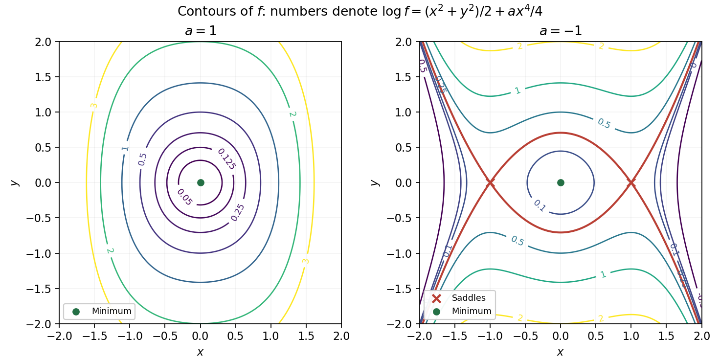
Because the exponential function is strictly increasing, the level sets are exactly those of . For they satisfyThere are no contours for , the level is the origin, and gives nested closed ovals symmetric about both axes. Their stronger fourth-power growth in makes them relatively narrower horizontally as the level rises.
For , the contour equation becomesThe central local minimum is surrounded by closed ovals for , accompanied by outer open branches. At , the level passes through the two saddle points and changes its connectivity. Levels have only outer branches, while levels above the saddle value have an upper and a lower branch. The sketch is restricted to the requested square; labels give , so they identify the corresponding contours of without exponentially large labels.


For , the local minimum at the origin has . Its full level set isThe connected component containing the minimum is just the isolated origin. The same level also has the outer branches for ; these are different connected components, not curves approaching the origin.
Articles were limited to the first 100 out of 155 total.
Articles by others on the same topic
There are currently no matching articles.