Translate the coordinates by and , and write . The partial derivatives areIf or , these equations together force . Otherwise they require . Thus the complete set of stationary points is
At the central stationary point, , so . At each of the other stationary points, and hence . Therefore
In the translated coordinates , , the zero level set is the pair of lines and . The function is positive in the quadrants and negative in those with , and tends to zero as . Thus its nonzero contours form closed curves around the four off-centre stationary points.
For an explicit description of the contour plot, use polar coordinates , :At fixed direction within a quadrant, the magnitude increases until and then decreases towards zero. Also , with equality exactly when , and similarly for . Consequently ; each positive level below encloses a positive peak in each positive quadrant, with the analogous negative contours in the negative quadrants.
To classify the stationary points, the Hessian matrix isAt it is , with eigenvalues and , so is a saddle point. At it is . Therefore and are strict local maxima, and and are strict local minima. These are also global maxima and minima by the bound just proved.
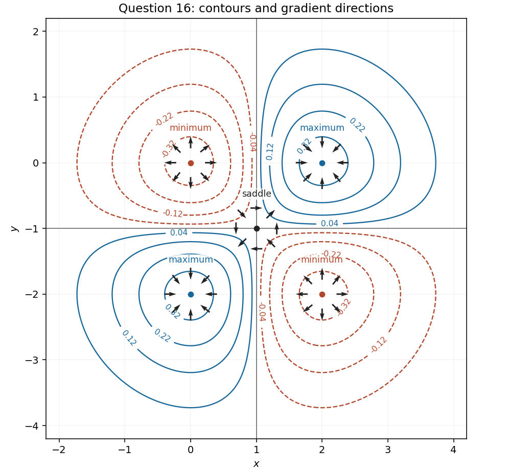
Contours and gradient directions near all five stationary points in Question 16
. Details. 
The gradient isIt is perpendicular to each nonzero level set and points towards increasing . Near the two positive local maxima, the Hessian matrix is , so the gradient arrows point inward. Near the two negative local minima, the Hessian matrix is , so they point outward. These arrows are shown on the figure in part (c).
At the saddle point, . Along , the arrows point away from the centre on both sides; along , they point towards the centre on both sides. On the positive axis they point up, on the negative axis down, on the positive axis right, and on the negative axis left. This specifies the four intervening sectors of the gradient pattern.
Articles by others on the same topic
There are currently no matching articles.