A scanning transmission electron microscope makes an image by assigning a transmitted-electron signal to each position of a scanned probe. Its essential chain is electron source, probe-forming optics, scan system, thin specimen, transmitted-electron detectors and synchronized acquisition.
An electron gun and accelerating supply provide a stable beam of the chosen kinetic energy. Condenser lens optics and an aperture control probe current and convergence; the probe-forming objective lens focuses a small spot on the specimen. Alignment, focusing and astigmatism correction keep the probe usable across the field.
Scan coils deflect the probe in a raster. A stable specimen holder positions an electron-transparent region, and a high-vacuum column limits gas scattering and contamination. A bright-field transmission electron microscopy detector collects the central transmitted beam; an annular detector can select annular dark-field electron imaging, including high-angle annular dark-field imaging. Different angular selections give different contrasts, rather than a universal map of height.
Detector electronics, scan timing and a computer assign the collected signal to the corresponding image pixel. Spectrometers are useful additions but not essential to basic image formation. The post-specimen optics can adjust detector collection geometry; they do not set scan-image magnification in the same way as the projection lenses of conventional transmission imaging.
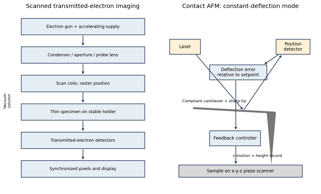
Original schematics of scanned transmitted-electron imaging and contact-mode force feedback; panels show different instruments
. Details. 
For a displayed width representing a scanned specimen width , the linear image magnification isThe user changes the scan-coil excursion, hence . A smaller raster displayed at the same width gives larger magnification. Changing the display or print size also changes displayed magnification, so the calibrated scale bar is more portable than a magnification label. This is the scan/display principle described in the manufacturer's microscope guide.[ref]
Scanning Electron Microscope A To Z by JEOL. Magnification of SEM, printed p.7: scan width and display width; the same raster-display geometry applies in STEM
At the low-magnification extreme, the probe scans the widest accessible field. Coil range, apertures, scan distortion and maintaining focus constrain the actual usable width. Formally increasing without bound would make arbitrarily small, but a real column has a finite accessible field.
At the high-magnification extreme, the scan covers a very small region. Formally makes diverge, but exactly zero scan width samples one location and supplies no spatial image. Electron microscope resolution, finite probe size, pixel spacing, drift, noise and specimen damage set the useful limit. Enlarging a field already sampled more finely than its resolvable information produces empty magnification, not new structural detail. For pixels across a field, the specimen sampling interval is ; this is distinct from the probe's spatial resolution.
Articles by others on the same topic
There are currently no matching articles.