A scanning transmission electron microscope makes an image by assigning a transmitted-electron signal to each position of a scanned probe. Its essential chain is electron source, probe-forming optics, scan system, thin specimen, transmitted-electron detectors and synchronized acquisition.
An electron gun and accelerating supply provide a stable beam of the chosen kinetic energy. Condenser lens optics and an aperture control probe current and convergence; the probe-forming objective lens focuses a small spot on the specimen. Alignment, focusing and astigmatism correction keep the probe usable across the field.
Scan coils deflect the probe in a raster. A stable specimen holder positions an electron-transparent region, and a high-vacuum column limits gas scattering and contamination. A bright-field transmission electron microscopy detector collects the central transmitted beam; an annular detector can select annular dark-field electron imaging, including high-angle annular dark-field imaging. Different angular selections give different contrasts, rather than a universal map of height.
Detector electronics, scan timing and a computer assign the collected signal to the corresponding image pixel. Spectrometers are useful additions but not essential to basic image formation. The post-specimen optics can adjust detector collection geometry; they do not set scan-image magnification in the same way as the projection lenses of conventional transmission imaging.
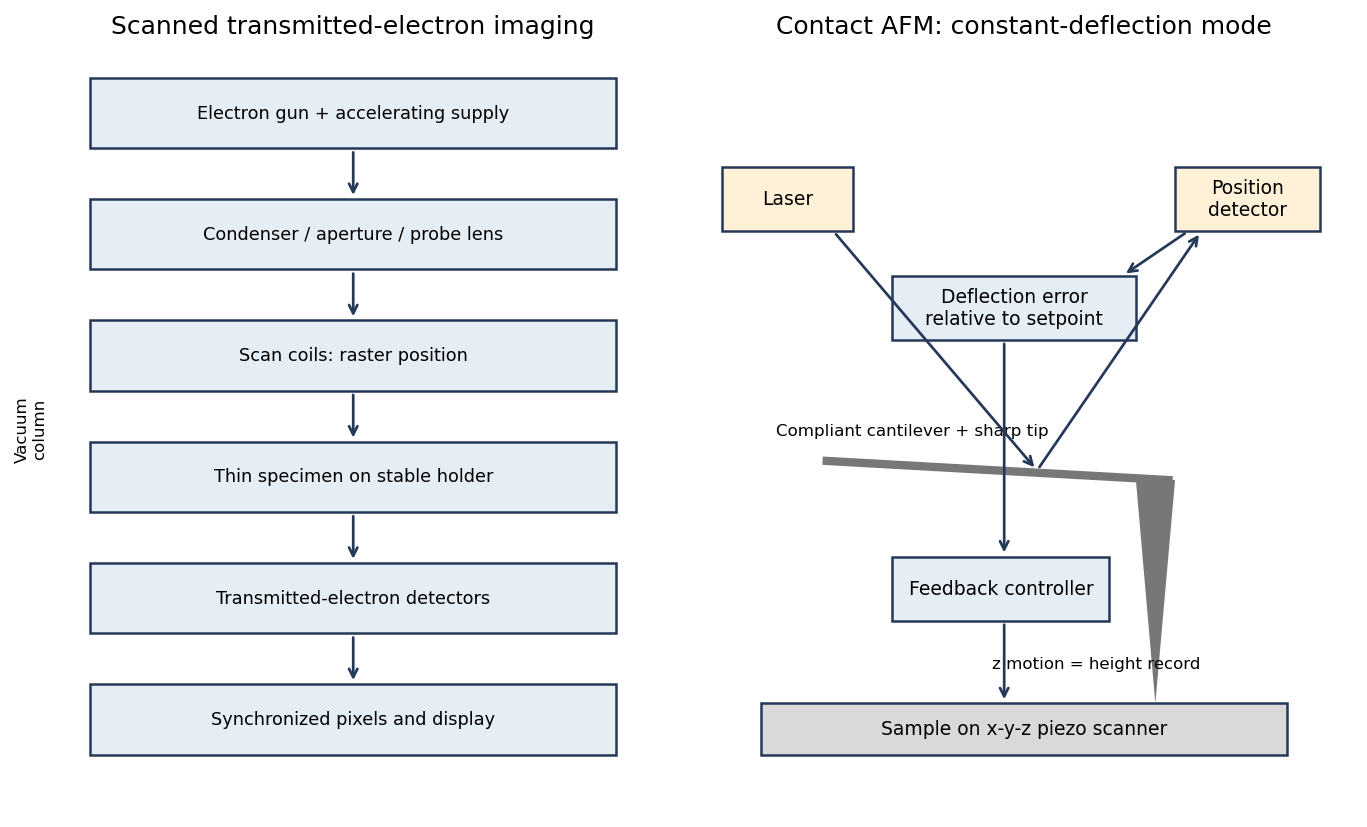
Original schematics of scanned transmitted-electron imaging and contact-mode force feedback; panels show different instruments
. Details. 
For a displayed width representing a scanned specimen width , the linear image magnification isThe user changes the scan-coil excursion, hence . A smaller raster displayed at the same width gives larger magnification. Changing the display or print size also changes displayed magnification, so the calibrated scale bar is more portable than a magnification label. This is the scan/display principle described in the manufacturer's microscope guide.[ref]
Scanning Electron Microscope A To Z by JEOL. Magnification of SEM, printed p.7: scan width and display width; the same raster-display geometry applies in STEM
At the low-magnification extreme, the probe scans the widest accessible field. Coil range, apertures, scan distortion and maintaining focus constrain the actual usable width. Formally increasing without bound would make arbitrarily small, but a real column has a finite accessible field.
At the high-magnification extreme, the scan covers a very small region. Formally makes diverge, but exactly zero scan width samples one location and supplies no spatial image. Electron microscope resolution, finite probe size, pixel spacing, drift, noise and specimen damage set the useful limit. Enlarging a field already sampled more finely than its resolvable information produces empty magnification, not new structural detail. For pixels across a field, the specimen sampling interval is ; this is distinct from the probe's spatial resolution.
A tip-change artefact occurs when the effective apex changes during scanning, for example through material pickup, loss of an attached particle or damage. In tapping-mode atomic force microscopy, a sudden change can introduce a false height offset between parts of the image, even on a continuous terrace.
The change alters the probe–surface interaction or the effective point at which the chosen amplitude setpoint is reached. The controller moves the vertical scanner to recover that setpoint, recording a spurious step or a change in line baseline. The sign is not fixed: different apex changes can move the apparent surface up or down.
The amplitude channel usually shows a transient deviation as the interaction changes; with stable feedback it returns toward its setpoint. It therefore need not retain the same persistent offset as the recorded height. A change in probe resonance or free amplitude can also change the operating condition. If the apex geometry has changed, widths and shapes can change too, or duplicated structures can appear as a double-tip artefact. A baseline correction cannot recover these lost geometric data.
AFM image flattening estimates an unwanted background and subtracts it from the recorded height:A plane removes overall tilt; a line-by-line constant or low-order fit removes line offsets or curvature. For a tip-change height jump, align the baselines of unchanged reference regions on either side of the event, using a piecewise offset or appropriately masked line fits. A single global plane cannot in general remove an abrupt step.
Exclude genuine features from the fit, use the same terrace as a reference where possible, and retain the unprocessed data. The corrected image has a consistent relative background; it does not establish that the interaction force, tip shape or absolute height calibration remained unchanged. In particular, flattening is a correction for the offset component of a tip-change artefact, not a repair of every consequence of a changed tip.
Sample tilt and scanner bow are other common backgrounds that AFM image flattening can remove. Fit a plane to a genuinely flat reference area and subtract it to remove tilt. A low-order curved fit can approximate the vertical background produced by a piezoelectric scanner's non-planar motion.
Line-dependent offsets or slow drift can sometimes be removed by subtracting a reference level from each scan line. Mask pits, particles and true steps so that they do not bias the reference. An independently measured flat calibration specimen and scans in different orientations help distinguish instrumental background from actual specimen curvature.
Flattening removes fitted components of the image whether they are instrumental or real. A true specimen slope, broad dome or slow height variation can be erased if it resembles the chosen background. Strong features can bias a fit and create false depressions, streaks or halos; an overly flexible polynomial can fit away scientifically useful topography.
Line-by-line correction can destroy real differences between terraces, especially when no common flat region spans the lines. Height statistics, roughness and feature depths then depend on masking and fit order. Report those choices and compare profiles before and after processing.
Flattening does not restore structures inaccessible to the tip, undo a double-tip artefact, remove finite-tip broadening, reconstruct a saturated signal or recover data lost to unstable feedback. It also does not calibrate the scanner. These limitations are important when a superficially smoother image is mistaken for a more accurate measurement.
Articles by others on the same topic
There are currently no matching articles.