Past exam of the MPhil in micro- and nanotechnology enterprise course of the University of Cambridge / 2020 / Paper 1 / Section B / 8

One image takes $512\mathrm{s}$ if $1\mathrm{Hz}$ means one completed scan line per second. The slow-axis speed is $10/512=0.01953\mu \mathrm{m}{\mathrm{s}}^{-1}$. Recording a wire spanning $1\mu \mathrm{m}$ along that axis therefore takes $51.2\mathrm{s}$. Meanwhile the fast-axis drift is $20/3600=0.005556\mu \mathrm{m}{\mathrm{s}}^{-1}$, giving a transverse displacement of $0.2844\mu \mathrm{m}$. The apparent straight-line length isIts slow-axis projection remains $1\mu \mathrm{m}$; the overestimate refers to length along the slanted trace.

With the wire along the fast axis and drift along the slow axis, its length is acquired within one line, so $L_{\mathrm{app}}\simeq 1.000\mu \mathrm{m}$. Taking a forward sweep of $1\mathrm{s}$ across $10\mu \mathrm{m}$, the wire is crossed in $0.1\mathrm{s}$ and the perpendicular displacement is only $0.556\mathrm{nm}$. The corresponding length change is about $1.5\times 10^{-7}\mu \mathrm{m}$, far below the $19.5\mathrm{nm}$ pixel pitch. For the convention in which one hertz includes a forward and reverse sweep, that already negligible displacement halves. The slow-axis calculation still uses one completed line per second.

Place the wire parallel to the fast scan axis. The endpoints are then recorded in a fraction of a line period, rather than tens of seconds apart, minimizing the differential drift accumulated between them.

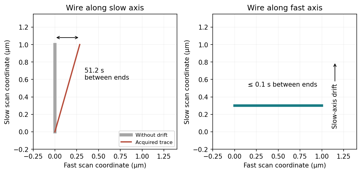
This does not remove drift of the wire's transverse position or apparent width between successive lines. A very thin wire parallel to the fast axis may fall between the discrete slow-axis scan lines, so a smaller scan area or denser sampling can be needed. Tip convolution, pixel resolution and feedback lag remain; trace/retrace comparisons and allowing thermal equilibration are still valuable. Increasing the scan speed indefinitely is limited by the scanner and feedback bandwidth.

Scanner bow is the relevant artefact. A piezoelectric tube scanner bends to produce lateral displacement; its moving end also follows a curved vertical trajectory. Cross-coupling of lateral and vertical motion therefore gives a roughly quadratic height background even over a flat reference. Over a wide scan it can mimic or conceal a genuine parabolic sample profile; its sign depends on scanner geometry and height convention.

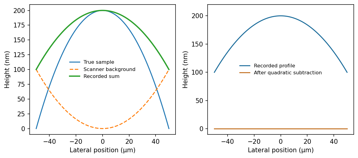
Common processing fits and subtracts a low-order polynomial background, often a quadratic surface or a polynomial for each scan line. This AFM image flattening removes scanner curvature on an assumed flat sample. Here the desired specimen signal is itself roughly quadratic, so such subtraction can remove the actual $200\mathrm{nm}$ bulge along with the artefact. The two contributions cannot be separated by polynomial fitting to this image alone. A plane subtraction removes tilt but does not independently calibrate curvature.

Measure a genuinely flat calibration reference over the same scan range, scanner position and operating conditions, then subtract its reproducible bow background from the specimen data. Retain reference flat regions outside the feature if available, fitting only those regions rather than the bulge. A scanner with independently measured vertical motion or suitable closed-loop correction reduces the instrumental uncertainty. Translating or rotating the specimen checks whether a feature follows the specimen or the scanner coordinates; independent optical or stylus profilometry can corroborate its height. For a rotationally symmetric parabola, rotation alone is not sufficient. Report drift and calibration uncertainty as part of the $200\mathrm{nm}$ height measurement.