Past exam of the perturbation methods and applied complex variables course of the University of Oxford / 2007 / A (Perturbation Methods)

Away from the boundary, derivatives of a smoothly varying solution are much smaller than $k^{2}f$ unless the outer solution vanishes. Nonzero boundary data therefore require a rapidly varying layer. If its thickness is $\delta$, the radial second derivative is of order $f/{\delta }^2$; balancing it with $k^{2}f$ gives $\delta =k^{-1}$.

Put $R=k(1-r)$ and write $f(r,\theta )=F(R,\theta )$. The equation becomesFor fixed $R$ and boundary data with angular variation independent of $k$, the leading equation is $F_{RR}=F$. Matching to the zero outer solution removes the growing exponential, and the boundary value at $R=0$ fixes its coefficient:This approximation describes the layer; it is not a uniform expansion in polar coordinates at the origin.

Laplace's method localizes an exponential integral near maxima of its real phase. At an isolated smooth interior maximum $t_0$ with $G^{\prime \prime }(t_0)<0$ and $F(t_0)\ne 0$, Taylor expansion and Gaussian integral giveAn endpoint maximum with nonzero inward phase slope instead gives an inverse-$k$ factor. Degenerate maxima require their first nonzero local phase term; continuous differentiability alone does not guarantee the quadratic formula.

Here $\cos (ix\sin \varphi )=\cosh (x\sin \varphi )$. In its two exponentials, the positive exponential dominates at the interior maximum $\varphi =\pi /2$ of $\sin \varphi$. Since $\sin (\pi /2+s)=1-s^2/2+O(s^4)$,The negative exponential has no comparable positive maximum and is negligible. Consequently, where $kr\to \infty$,In the boundary layer $r=1-R/k$, $r^{-1/2}=1+O(k^{-1})$, so this reduces to $e^{-R}$, agreeing with the formal result when $g=1$.

Define $y=k^{-1}\dot{x}+x^3/3-x$. Differentiation and the original equation give $\dot{y}=(\lambda -x)/k$, while rearrangement gives $\dot{x}=k(y-x^3/3+x)$. Write $h(x)=x^3/3-x$.

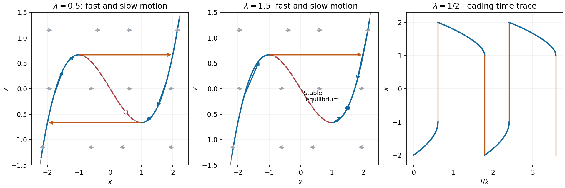
On the fast scale $\tau =kt$,Fast trajectories are horizontal. Their equilibria lie on the cubic $y=h(x)$; the transverse linearization is $-h^{\prime }(x)=1-x^2$, so the outer branches $|x|>1$ attract and the middle branch repels. On a horizontal line, arrows point right when $y>h(x)$ and left when $y<h(x)$.

The source prints the slow time as $T=k/t$. The slow variable needed here is $T=t/k$. With this correction,At leading order $y=h(x)$ andThe reciprocal printed variable would give $-T^2{y}_T=\lambda -x$, rather than the autonomous slow equations used in the stated period formula.

For $-1<\lambda <1$, the left attracting branch runs from $x=-2$ to the fold $x=-1$, where $y=2/3$. The horizontal fast jump at this height lands at $x=2$. The right branch then runs from $2$ to the fold $1$, where $y=-2/3$, followed by a fast jump to $-2$. The equilibrium at $x=\lambda$ is on the repelling middle branch. The two slow segments dominate the period:The jump times are negligible on this $O(k)$ scale. Substituting $u=-x$ in the first integral also gives the compact valueFor $\lambda =1/2$, the negative slow segment takes $k[1-\frac{3}{4}\log (5/3)]$, and the positive one takes $k[2-\frac{3}{4}\log 3]$. Thus $x(t)$ rises slowly from $-2$ to $-1$, jumps to $2$, decreases more slowly to $1$, then jumps back to $-2$; the jumps are nearly vertical in the time trace.

For $\lambda >1$ the fast horizontal field and attracting branches are unchanged. The right slow branch has arrows toward $x=\lambda$ from both directions; the left branch still moves toward $-1$ and jumps right. The equilibrium $(\lambda ,h(\lambda ))$ is stable, so the large relaxation cycle is replaced by approach to this equilibrium. If $\lambda >2$, a landing at $2$ moves right toward $\lambda$, rather than left. The sketches display the representative case $\lambda =3/2$.

For fixed nonzero $x$, expand the denominator geometrically:The effective expansion parameter is ${ϵ}^2/x^2$, so the expansion fails when $x=O(ϵ)$. In the inner variable $X=x/ϵ$,for fixed $X$. Expanding the leading outer term toward $x=0$ gives $x^{-2}$ at leading order; expanding the leading inner term for large $X$ and returning to $x$ gives ${ϵ}^{-2}{X}^{-2}=x^{-2}$. Thus the two one-term re-expansions match in $ϵ\ll x\ll 1$. The next common contribution is $-x^{-1}$ when the corresponding next inner order is retained.

On $x\ge \delta$, the relative denominator error is bounded by ${ϵ}^2/{\delta }^2$, henceIntegration by parts yieldsFor the last step split the remaining integral at one: ${\int }_{\delta }^{1}dx/x=-\log \delta$, and replacing $e^{-x}$ by one on that interval has a bounded error.

In the inner interval, $|e^{-x}-1|\le x$ gives an explicit error estimate:The $1/\delta$ terms cancel between regions. Every displayed remainder is $o({ϵ}^{-1})$ whenever $ϵ/\delta \to 0$ and $\delta \to 0$; for example $ϵ({ϵ}^2/{\delta }^3)=(ϵ/\delta {)}^3$. Therefore the leading answer is independent of the arbitrary intermediate cutoff:

On the two independent variables, the total derivative is $D_x={\partial }_x+{ϵ}^{-1}{\partial }_X$. Multiplication of $D_x(a{D}_{x}y)=f$ by ${ϵ}^2$ gives exactly the stated multiple-scale equation.

At order one, ${\partial }_X(a{\partial }_X{y}_0)=0$. Integrating twice givesThe periodic reciprocal coefficient has strictly positive mean. Unless $A=0$, the integral has a nonzero linear drift in $X$, violating the periodic cell ansatz and creating secular growth when $X=x/ϵ$. Thus $A=0$ and $y_0=y_0(x)$.

At order $ϵ$,Periodicity requires the derivative to have zero cell average. ConsequentlyAt order ${ϵ}^2$, the equation isThe second flux inside braces is $C(x)$, independent of $X$. Integrating over one period annihilates the first derivative, by periodicity, and yields $C^{\prime }(x)={\int }_0^{1}f(x,X)dX$. HenceThe effective transport coefficient is the harmonic mean of $a$ over the fast period; the source is averaged arithmetically. Smoothness sufficient for these formal differentiations and uniform positivity on the cells are understood.