Away from the boundary, derivatives of a smoothly varying solution are much smaller than unless the outer solution vanishes. Nonzero boundary data therefore require a rapidly varying layer. If its thickness is , the radial second derivative is of order ; balancing it with gives .
Put and write . The equation becomesFor fixed and boundary data with angular variation independent of , the leading equation is . Matching to the zero outer solution removes the growing exponential, and the boundary value at fixes its coefficient:This approximation describes the layer; it is not a uniform expansion in polar coordinates at the origin.
Laplace's method localizes an exponential integral near maxima of its real phase. At an isolated smooth interior maximum with and , Taylor expansion and Gaussian integral giveAn endpoint maximum with nonzero inward phase slope instead gives an inverse- factor. Degenerate maxima require their first nonzero local phase term; continuous differentiability alone does not guarantee the quadratic formula.
Here . In its two exponentials, the positive exponential dominates at the interior maximum of . Since ,The negative exponential has no comparable positive maximum and is negligible. Consequently, where ,In the boundary layer , , so this reduces to , agreeing with the formal result when .
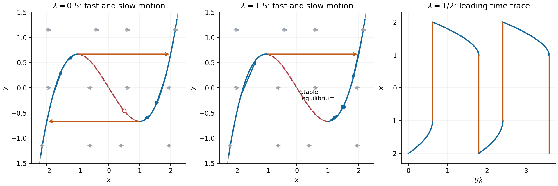
On the fast scale ,Fast trajectories are horizontal. Their equilibria lie on the cubic ; the transverse linearization is , so the outer branches attract and the middle branch repels. On a horizontal line, arrows point right when and left when .
The source prints the slow time as . The slow variable needed here is . With this correction,At leading order andThe reciprocal printed variable would give , rather than the autonomous slow equations used in the stated period formula.
For , the left attracting branch runs from to the fold , where . The horizontal fast jump at this height lands at . The right branch then runs from to the fold , where , followed by a fast jump to . The equilibrium at is on the repelling middle branch. The two slow segments dominate the period:The jump times are negligible on this scale. Substituting in the first integral also gives the compact valueFor , the negative slow segment takes , and the positive one takes . Thus rises slowly from to , jumps to , decreases more slowly to , then jumps back to ; the jumps are nearly vertical in the time trace.
For the fast horizontal field and attracting branches are unchanged. The right slow branch has arrows toward from both directions; the left branch still moves toward and jumps right. The equilibrium is stable, so the large relaxation cycle is replaced by approach to this equilibrium. If , a landing at moves right toward , rather than left. The sketches display the representative case .
For fixed nonzero , expand the denominator geometrically:The effective expansion parameter is , so the expansion fails when . In the inner variable ,for fixed . Expanding the leading outer term toward gives at leading order; expanding the leading inner term for large and returning to gives . Thus the two one-term re-expansions match in . The next common contribution is when the corresponding next inner order is retained.
On , the relative denominator error is bounded by , henceIntegration by parts yieldsFor the last step split the remaining integral at one: , and replacing by one on that interval has a bounded error.
In the inner interval, gives an explicit error estimate:The terms cancel between regions. Every displayed remainder is whenever and ; for example . Therefore the leading answer is independent of the arbitrary intermediate cutoff:
On the two independent variables, the total derivative is . Multiplication of by gives exactly the stated multiple-scale equation.
At order one, . Integrating twice givesThe periodic reciprocal coefficient has strictly positive mean. Unless , the integral has a nonzero linear drift in , violating the periodic cell ansatz and creating secular growth when . Thus and .
At order ,Periodicity requires the derivative to have zero cell average. ConsequentlyAt order , the equation isThe second flux inside braces is , independent of . Integrating over one period annihilates the first derivative, by periodicity, and yields . HenceThe effective transport coefficient is the harmonic mean of over the fast period; the source is averaged arithmetically. Smoothness sufficient for these formal differentiations and uniform positivity on the cells are understood.
Choose each factor with its argument between zero and in the upper half-plane. On an interval between consecutive real prevertices, each factor has a constant boundary argument, so has constant argument and the image is a straight side. Crossing from left to right decreases by , hence increases by , giving the prescribed exterior turn. Locally,so an upper half-disc maps to angle , the required interior angle. The overall constant rotates and scales the polygon; integration adds translation. For a general prescribed polygon, the prevertex positions must also satisfy the side-length conditions: the derivative formula fixes angles but arbitrary choices do not fix arbitrary side lengths.
For the slit domain, the slit tip has interior angle , so its exterior parameter is . The two vertices at infinity give the factors at , leading to proportional to . Integrating and imposing the tip value givesThe square root is the principal one: for , never lies on the nonpositive real axis. Thus . Boundary points map to the two banks of the slit, with at the tip; the outside intervals map to the imaginary axis. The derivative is nonzero in the open half-plane. Conversely each point of the slit domain determines exactly one root of with positive imaginary part, proving bijectivity.
The Möbius map takes the upper half-plane to itself, so its principal argument lies in . The imaginary part of its analytic logarithm is harmonic, equals on and zero on the other real intervals. ThusIt lies between zero and one and has the required boundary limits away from the two discontinuities. Pulling this harmonic function back by the inverse conformal map yieldsThis specifies all branches and remains bounded even as tends to either end at infinity.
To exhibit nonuniqueness without the growth restriction, putThis is harmonic in the domain. On its boundary the corresponding is real and the rational expression is real, except at , which represent infinity. At , representing , the expression tends to zero. Thus has zero finite boundary data. It is nonzero, since for its value is , and it is unbounded as approaches either pole non-tangentially. Therefore gives distinct solutions with the same finite boundary data when boundedness at infinity is removed.
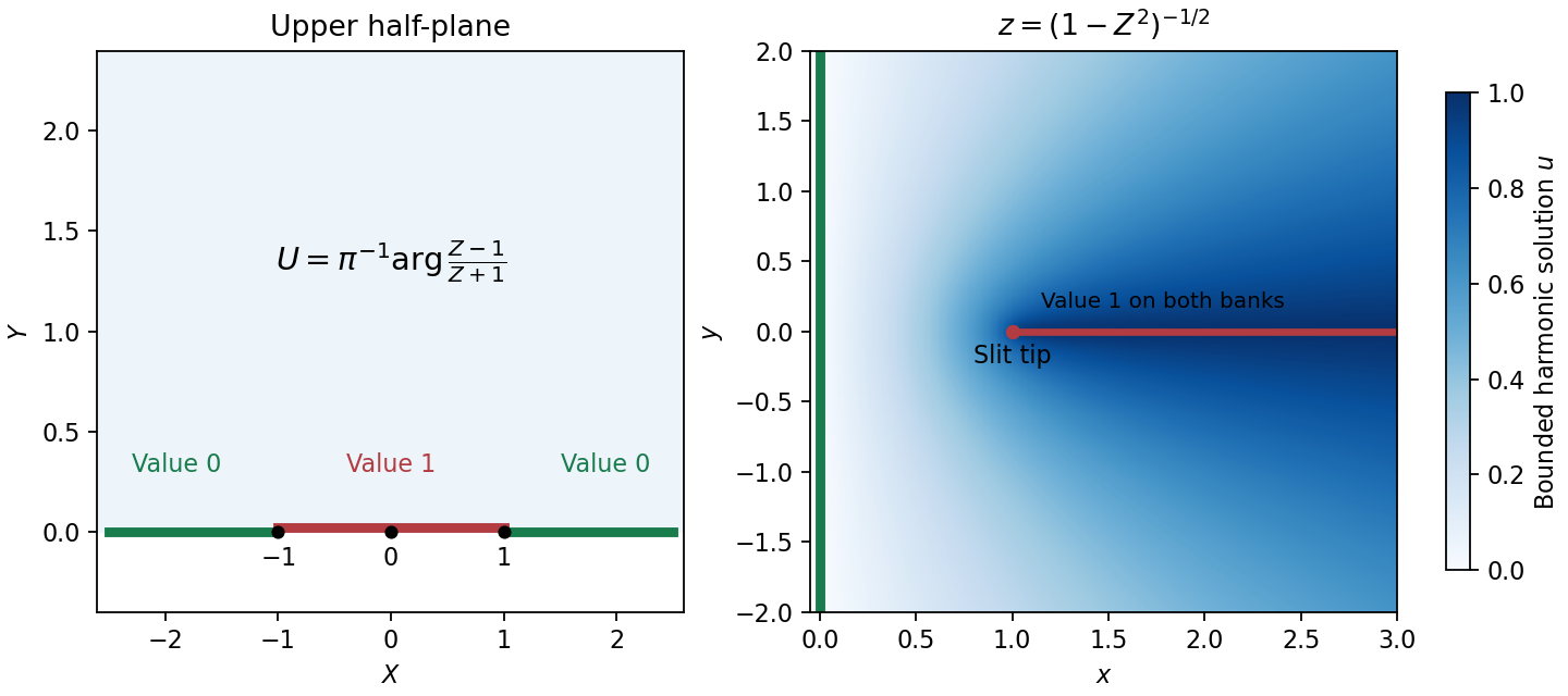
Prevertices, the slit domain, and the bounded harmonic boundary values
. Details. Conformality implies , so . Apply the stated Green's theorem with :Here on the unit circle. The lowest power in is , while the most negative power in the conjugate polynomial is . For their product has no term. The residue theorem gives for all .
When , the residue for is . For , expandOnly contributes. ThereforeThe first is the area; the second records its complex first moment, and need not be real.
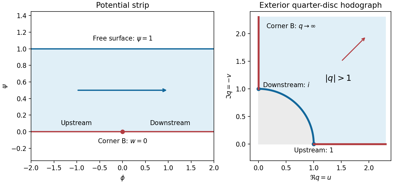
The potential plane is the strip . The wall maps to its lower boundary, with upstream , the corner at , and downstream . The free surface maps to its upper boundary.
Write . Far upstream ; far downstream the flow points vertically down and . On the two wall rays, runs along the positive real and positive imaginary axes. The reentrant fluid corner has angle , so its potential behaves locally as and its speed diverges like . Thus the corner corresponds to , not . The free surface has , giving the hodograph domainIt is the exterior of a quarter unit disc in the first quadrant.
Now maps this domain to the part of the upper half-plane outside the unit disc. The maptakes it to the first quadrant: its real and imaginary parts are positive because and . Finally maps that quadrant to the upper half-plane. The corresponding strip map is . Both give upstream , corner , and downstream , so the three boundary normalizations fix the remaining real Möbius freedom. ConsequentlyOn the free surface , , so is negative and as required. On the wall , giving .


The integral construction requires differentiation under the integral and vanishing boundary terms. With those assumptions, integration by parts givesThe standard construction therefore sets , giving . Convergent contours run between rays where : convenient central rays have arguments , and . Two choices are the oriented pathsThe cubic exponential dominates the linear one at both ends. To verify independence directly, put and . At the value and derivative of the integral along rays are and . For the two contours above their derivative-to-value ratios are respectively and , which differ. Hence their Wronskian is nonzero.
For the second equation multiply by before integrating by parts:Setting the residual weight to zero gives . One contour is the segment from to , with the square root positive at . Its integral is a nonzero multiple of : substituting gives , an entire function nonzero at zero.
A second contour starts at and follows , , choosing a continuous branch along the path. For it converges at infinity; at the branch endpoint its integrable singularity is . In both cases the boundary term contains and vanishes at branch endpoints. The second integral has a nonzero logarithmic divergence as through positive real values, because its large- integrand is a nonzero multiple of . It is therefore independent of the entire first solution; analytic continuation supplies solutions elsewhere away from the equation's singular point.
Strictly, nonzero and an arbitrary contour alone do not prove the printed necessity for . Necessity also needs injectivity of the chosen Laplace representation, while the vanishing-integrand argument above is the usual sufficient construction. For a concrete counterexample to unconditional necessity in the Bessel case, take a positively oriented circle , choose the branch outside the cut , and add one to that weight. The added entire integrand integrates to zero. Expanding the original weight on this circle gives integral , which is nonzero and solves the equation, although the modified weight is not a constant multiple of the printed one. The standard weights and contours above still give the requested independent solutions.
Letbe the root with positive real and positive imaginary parts. More explicitly, with ,Decay at each infinity and continuity at zero force for and for . The derivative jump is , soThe two roots lie in the first quadrant, so their sum cannot vanish.
Integrating the differential equation twice by parts on each half-line givesTheir sum is the stated identity with right side one. Equivalently the global distributional equation is , since the derivative has jump one.
The direct half-transforms areHere is analytic above its lower-half-plane pole , while is analytic below its upper-half-plane pole .
To recover the same result from the transform identity alone, use Wiener-Hopf factorization:Multiply by . The coefficient of becomes , analytic and zero-free in the lower half-plane, while the coefficient of is analytic and zero-free in the upper half-plane. Split the right side asThe first term is analytic above and the second below. Equating the separated functions and using their decay at infinity fixes the entire remainder to zero, yielding the boxed , with the branches fixed before factorization.
There are two distinct inconsistencies in the printed formulas. First the initial Cauchy integral has coefficient , whereas the stated boundary limits require . Second the final integral is a solution of a difference jump problem, although the intervening equation for is a sum jump problem. We derive the valid identities, show precisely where that final deduction fails, and give the corrected construction. Take and, initially, a Hölder continuous density on the interior with integrable endpoints, so the boundary limits and principal values exist.
Define the Cauchy principal value byFor the corrected normalization , subtract from the numerator near . The subtracted integral has the common principal-value limit, while integration of the remaining constant density produces boundary arguments differing by . This proves the Sokhotski–Plemelj theoremIn particular and . With the literal printed integral instead, the limits are , and the next stated boundary equation would have right side .
Use the corrected normalization from now on and write , , . The original singular integral equation then becomesIf satisfies the printed homogeneous relation , division of gives, correctly,A nonvanishing factor is needed as well as the printed nonvanishing of ; its zeros would require separate treatment.
The next printed step is invalid because a Cauchy integral of has boundary difference , not boundary sum . A particularly direct counterexample is , , . The original equation is simply . Choose , with at infinity and cut . Its boundary values are , so it satisfies precisely the printed homogeneous sum relation. But the printed proposed integral yieldsThe integral follows by , or the usual elementary integral . Its proposed is constant, has jump zero, and is not the Cauchy transform of ; it also fails the required decay at infinity. If the printed is interpreted as principal value in its last formula, that value is zero, giving and the same contradiction.
To solve the sum jump correctly, introduce this sign-changing factor . Set , soThe corrected local Cauchy representation is consequentlyHere has no jump across the open interval; its possible endpoint singularities and polynomial part are determined by endpoint admissibility, absence of unwanted poles, and at infinity. Some choices of factor require a weighted or regularized integral at the endpoints. Thus nonvanishing of alone does not determine a unique global solution without a function class and growth conditions.
Equivalently put . It satisfies the homogeneous difference relation . If , , and the integral is admissible, thenTaking its jump gives the usable density formulaThis formula, together with the endpoint and infinity conditions, replaces the last printed equation. Alternatively, if the homogeneous relation in the question is changed from plus to minus, its unweighted Cauchy representation becomes a valid particular solution, but the density must still be obtained from this jump calculation and homogeneous terms still require normalization. The statements cannot all hold simultaneously as printed.
Articles by others on the same topic
There are currently no matching articles.