Section C: Geophysical Methods.
A gravity anomaly is measured gravitational acceleration, reduced to a stated reference surface and compared with a reference gravity field. A local geological interpretation further removes or models the regional background. An absolute negative Bouguer gravity anomaly is therefore not itself a local negative geophysical density contrast.
Measure relative gravity with a calibrated gravimeter at stations across the profile, tie it to a base station, repeat base readings to estimate instrumental drift, and measure station coordinates and accurate elevations, for example by GNSS and levelling. Record observation times for tide corrections. Subtract the latitude-dependent reference gravity, correct instrument drift and Earth tides, add the free-air correction for station height, and subtract the attraction of the reference-density Bouguer slab. A terrain correction accounts for relief missing from or exceeding that slab. Use a consistent density such as for the topographic correction.[ref]
Geophysical Data Grids for the Conterminous United States by United States Geological Survey. Gravity anomaly reduction: free-air, simple-Bouguer and complete-Bouguer corrections
The question's reference to the anomaly in panel b is a panel-label slip: the upper plot contains gravity, while the lower plot supplies geometry and elevations. A geological slab thickness is the vertical thickness of the anomalous body, not simply its height above sea level.
For a laterally extensive Bouguer slab of thickness and geophysical density contrast ,The greenstone belt reaches from roughly to near its deepest central part, so use . The gravity maximum is approximately ; the exposed host-rock background in the south is approximately . Taking this as a constant regional reference gives a local excess . ThusThis is an approximate density under a constant-background, infinite-slab model. The finite width, variable thickness and neighboring pluton require a fuller gravity inversion for a precise value. In particular, the absolute value must not be inserted as the local excess.
Retain the same regional-background assumption as in part (b). The northern pluton is about thick beneath the station near the northern trough, while its gravity anomaly is about . Its anomaly relative to the greenstone maximum is approximately . Therefore the contrast equation isUsing the result of part (b), the second term contributes , leaving a net pluton anomaly of about . Hence , effectively close to the host-rock density at the precision of this diagram.
The apparent trough is strongly negative relative to the greenstone belt, but hardly negative relative to the southern host-rock background. If a northward regional trend is intended instead, it must be stated: in general,with both gravity values in milligals. For example, a northern background of would give , but the same reference would also change part (b). No regional curve is explicitly identified in the supplied figure, so the numerical result must retain its reference-field assumption. This is the geological nonuniqueness of geophysical inversion of potential-field interpretation, rather than a reason to force a presumed textbook granite density onto the plot.
Measure total magnetic field along the same south–north line with a calibrated magnetometer, recording position, time and sensor height. A simultaneous base-station magnetometer measures temporal variation so that diurnal changes can be removed from the moving survey. Avoid disturbed periods and magnetic contamination from vehicles, fences, power lines and equipment. Choose station spacing much smaller than the expected anomaly width, for example tens to hundreds of metres for a kilometre-scale target.
Subtract the epoch-appropriate International Geomagnetic Reference Field or another stated regional main-field model to obtain a total-field magnetic anomaly. Level overlapping traverses and remove offsets or drift where appropriate. Accurate terrain/sensor geometry is needed for comparison with a geological model, but there is no universal magnetic analogue of a constant-density Bouguer slab correction: the effect depends on the distribution and direction of magnetization. Measure magnetic susceptibility and remanent magnetization on representative greenstones, granite and host rock to test the assumed magnetic sources.
Assume the greenstone belt is more magnetically susceptible than the host rocks and granite, its magnetization is mainly induced magnetization, and the body is roughly east–west elongated so that the south–north line crosses it. At southern magnetic latitudes the main field has negative magnetic inclination in a north-and-down coordinate convention. The total-field magnetic anomaly is then generally asymmetric: the principal negative lobe is on the southern side and the positive lobe is displaced northward for the simple induced source illustrated here. The exact lobe sizes and peak positions depend on body geometry and the actual magnetic inclination.[ref]
Magnetic line profiles by UBC Geophysical Inversion Facility. Examples 1–2: the low lies north at northern inclination and south at southern inclination
An explicit sketching model is an induced magnetic dipole at depth . With northward coordinate , and unit field direction , its normalized total-field magnetic anomaly isThe plot uses only as an illustrative dipole-field inclination for a latitude near south, not a measured modern field at the site. A wide greenstone belt would broaden the response and can produce prominent edge anomalies. Remanent magnetization or a magnetic granite could change the sketch substantially; gravity alone cannot identify the magnetic source.
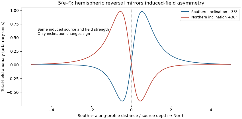
Induced-source magnetic anomalies for opposite inclinations on a south–north profile
. Details. 
For the same geometry, field strength and induced magnetization model at the opposite magnetic inclination, replacing by gives . Thus the north–south asymmetry reverses: the principal low moves to the northern side and the high to the southern side. It is a horizontal reflection of the simple profile, rather than a necessary reversal of every anomaly's sign. At a magnetic pole the induced anomaly is symmetric; at the magnetic equator the symmetry is different again. If remanent magnetization dominates, a hemisphere change alone does not determine the new profile because that remanence direction also has to be specified.
Articles by others on the same topic
There are currently no matching articles.