Worked solutions for the held Oxford second-year Earth Sciences examination of 1 June 2023. Source release: released question paper and Attachments A and B. The examination asks candidates to choose one question from each of six sections; every available numbered alternative is addressed here. These are derived solutions, with no question statements reproduced.
Source gap: Attachment C, referenced for Question 9, is absent from the held release. The printed summary table permits numerical calculations, but parts 9(d–e) remain explicitly provisional until that attachment and any conventions it supplied are checked. Attachments A and B are available and are treated as supporting material for Questions 3 and 4. Image positions below use fractions of the map frame, excluding page margins. The repeated salt-velocity subscript in Question 6 and the circular reference in Question 10 are documented where they affect the solution.
The fault dips are approximately . The mapped senses of fault slip are predominantly strike-slip faulting. In an Andersonian faulting regime, the intermediate principal stress is vertical and the maximum and minimum principal stresses are horizontal, so the preferred fault planes are vertical. Local bends can introduce oblique-slip faulting without changing this first-order interpretation.
Treat the two strands as newly formed conjugate faults obeying the same Mohr-Coulomb failure criterion, rather than merely inherited faults reactivated in a later stress field. A fault strike is an unoriented line, so is equivalent to . The acute angle between the fault strikes is therefore . The formal compressive acute bisector puts at azimuth and at . This orientation must also be checked against the mapped senses of strike-slip faulting, as discussed below.
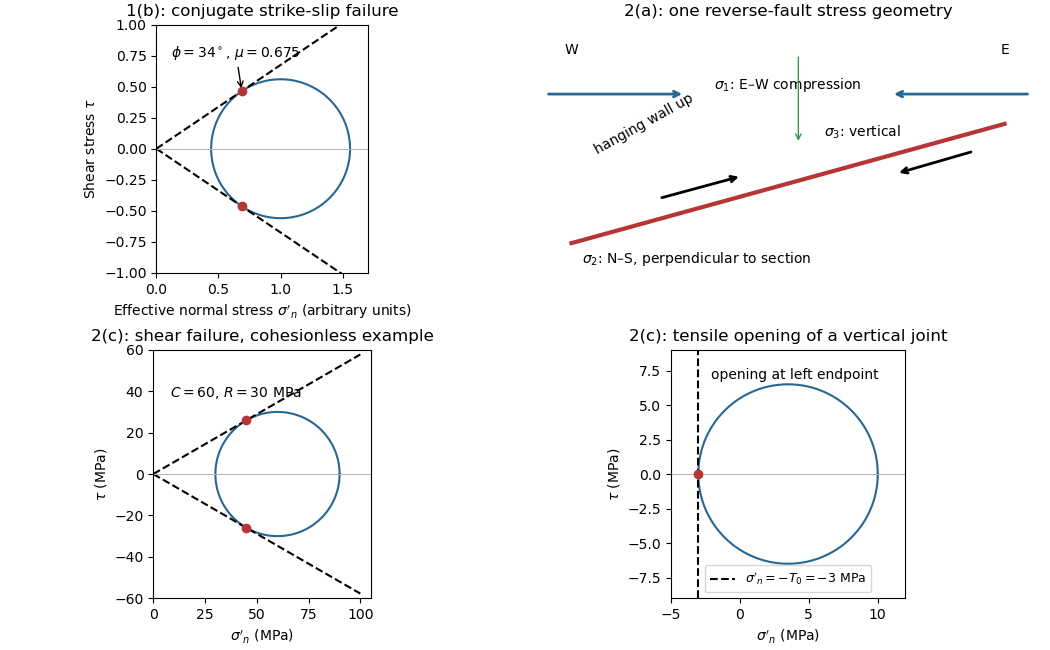
Let be the angle between either fault plane and . Tangency of Mohr's circle to , where is effective stress normal to the plane and is cohesion, gives and . ThusIn the Mohr circle, the fault planes are apart around the circle, because a physical plane rotation is doubled. The figure uses to display both tangencies; a common nonzero cohesion changes the intercept, not the inferred friction angle. The inference of requires optimally oriented conjugate faults at formation: the two fault strikes alone cannot measure a friction coefficient for arbitrarily reactivated faults.
Consistency limitation: the mapped westward motion of the Anatolian block corresponds to left-lateral strike-slip faulting on the East Anatolian strand and right-lateral strike-slip faulting on the North Anatolian strand. East–west maximum compression for the acute-bisector construction instead predicts the opposite pair. The stress orientation compatible with the mapped senses lies near the north–south, obtuse bisector; the planes are then about from , which would give in the optimal-formation formula. A negative friction angle is inadmissible for ordinary frictional strength. Thus is the formal magnitude inferred from unoriented angles, while the full map does not support a self-consistent positive-friction, optimally formed conjugate pair. The common-stress assumption can still describe inherited or anisotropically controlled faults, but then their orientations no longer determine a unique coefficient.

For a heterogeneous fault slip distribution, seismic moment iswhere is the shear modulus, the fault plane area, and the area-averaged fault slip. The peak colour cannot be used as : most of the illustrated fault plane has much smaller fault slip.
One reproducible graphical estimate divides the approximately long and down-dip panel into seven strips and a final strip. Reading area averages from the colour scale, from southwest to northeast, gives roughly . This includes the pale, nearly unslipped lower part of each strip. Henceand . A reasonable graphical range is approximately –, dominated by colour averaging and the down-dip extent of small fault slip. The corresponding moment magnitude is about , using . This is an estimate from the supplied distribution, rather than a substitution of a catalogued earthquake magnitude.
Effective stress and frictional strength generally increase with depth through the shallow crust undergoing brittle fracture. At , small overburden and often weak, fractured near-surface materials limit the shear stress and elastic energy that can accumulate. Some shallow materials also undergo stable sliding rather than unstable earthquake nucleation. Near , a locked fault prone to brittle fracture can sustain a much larger differential stress before frictional instability releases stored elastic energy.
This depth is plausibly near the lower, strong part of the seismogenic layer: below it, increasing temperature eventually promotes material creep across the brittle-ductile transition. Once nucleated at depth, a dynamic finite-source rupture can propagate into shallow regions that could not independently nucleate the same event. Depth alone does not determine the nucleation point: local pore pressure, frictional stability and stress heterogeneity also matter.
The star is near the southwestern end of the main fault slip patch, so a much longer part of the finite-source rupture propagates northeastward. For comparable distances, ground conditions and buildings, the northeastern site receives the stronger, shorter direct pulse; the southwestern site receives the weaker, longer direct shaking. This is rupture directivity.[ref]
What is Directivity by United States Geological Survey. Explanation of focusing by successive rupture elements
For a segment of length , rupture velocity and seismic wave speed , successive arrival times span approximatelyForward arrivals overlap and concentrate energy into a shorter pulse. Backward arrivals spread out. The supplied finite-source rupture is not perfectly unilateral, so the prediction concerns the dominant contribution. Seismic radiation patterns, seismic attenuation, sediment amplification and building response can alter the ranking of actual damage or total coda duration.
The offset layered sequence indicates reverse slip on the west-dipping fault: its western hanging wall moved up relative to the eastern footwall. With the fault strike perpendicular to the east–west image plane, an Andersonian faulting regime has horizontal east–west, horizontal north–south, and vertical. Draw opposing compression arrows east–west and a smaller opposing pair vertically; the intermediate pair points into and out of the page.
For example, in east, north, up coordinates, a compression-positive effective stress tensor consistent with a reverse fault and zero cohesion isThese magnitudes illustrate one possible stress tensor, rather than a measurement from the photograph. With , the – Mohr circle is tangent to the Mohr-Coulomb failure criterion at a plane from horizontal. The original failure-mechanics figure above sketches these principal stress directions.
Interpret the vertical, apparently unoffset fractures as opening geological joints. Their normals are east–west, so the least principal stress must be east–west and sufficiently tensile in effective stress. The other two principal stresses lie within the vertical north–south geological joint plane; their ordering cannot be recovered from this fracture orientation alone.
One example, with compression positive and coordinates east, north, up, isHere is vertical, north–south, and east–west. The geological joint opens east–west when its tensile strength is . An isotropic pore pressure can make the east–west effective stress tensile even while the total normal stress remains compressive. Draw opening arrows pointing away from the vertical fracture, rather than sliding arrows along it.
Use compression-positive effective stress normal to the plane on the horizontal axis and shear stress on the vertical axis. For any chosen pair of principal stresses, Mohr's circle has centre and radius .
For the reverse fault example, and . Draw the two Mohr-Coulomb failure criterion lines . The tangencies areThese are shear failure points with nonzero shear stress. The two smaller three-dimensional Mohr circles use and ; they lie inside the outer circle and do not touch the envelope in this example.
For the opening geological joints, use the tensile failure criterion . The example gives , and . The circle first touches this vertical cutoff at . Thus the geological joints form on planes normal to and have zero resolved shear stress. A complete brittle envelope can combine this tensile cutoff with compressive Mohr-Coulomb failure criterion, using sufficient cohesion that shear failure does not occur first. The failure-mechanics figure displays these two distinct constructions.
The reverse fault requires strong east–west compression; the vertical opening geological joints require the least principal stress in the effective stress tensor east–west. They need not have formed at the same time or under the same local stress field. Compression can form the reverse fault during burial and crustal shortening; subsequent tectonic exhumation, unloading, relaxation, cooling or another tectonic episode can rotate the principal stress ordering and permit opening geological joints.
Furthermore, local stress near faults, layer interfaces and topography can differ from the regional stress. A high pore pressure shifts every Mohr circle left by , helping tensile failure, but isotropic pore pressure alone cannot exchange the east–west and vertical principal stress ordering. Determine relative timing using cross-cutting relations, offsets of geological joints, and any generations of fracture-filling minerals. Spatial coexistence is therefore evidence of a deformation history, rather than a requirement that the two failure diagrams describe one simultaneous homogeneous stress state.
Within a shallow fault zone undergoing brittle fracture, repeated sliding crushes and grinds grains. Expect fault gouge, potentially rich in fine clay minerals, and coarser angular fault breccia; a cohesive, cemented crushed rock is a cataclasite. Slickensides or displaced grains can record the sliding direction.
An opening geological joint need not contain any fault rock: it may be an open crack. If fluids circulated, it can contain a mineral vein, for example calcite or quartz, grown from the fracture walls. Thus comminuted fault rock supports shear, while open space or a crack-filling mineral vein supports opening. Mineral filling is conditional on fluid chemistry and timing; its precise composition cannot be inferred from the photograph.
Section B: Remote Sensing and Active Tectonics.
Use calibrated multispectral imaging of reflected sunlight, with visible, near-infrared and short-wave-infrared bands. A satellite records radiance in several passbands for each ground pixel. Perform geometric registration and atmospheric correction to estimate spectral reflectance, then account for illumination differences on slopes and mask cloud, water and dense vegetation. A false-colour composite, diagnostic band ratios or a trained statistical classification can separate surface lithologies; field observations and representative spectra validate any mapped contact.
Different minerals have different absorption features: iron-bearing materials affect visible/near-infrared spectral reflectance, while hydroxyl-bearing clay minerals and carbonate-bearing rocks can differ in short-wave-infrared bands. Adjacent patches with reproducibly different spectra and coherent geological boundaries are candidates for lithological contacts. This is particularly useful in dry, exposed terrain. Vegetation, soil cover, similar rock compositions, weathering and topographic shadow can hide or mimic a contact; a colour boundary alone is insufficient.
Choose spatial resolution appreciably finer than the narrowest unit being mapped, with several pixels across that unit. Approximately – is suitable for regional contacts separated by hundreds of metres; metre-scale units require finer imagery or field work. Sentinel-2 provides – bands useful for this purpose, while the reflected-light multispectral bands of Landsat are typically . Broad multispectral passbands distinguish many rock assemblages but cannot resolve every narrow mineral absorption feature; hyperspectral imaging is preferable when those features are essential.
A displaced drainage forms when repeated horizontal fault slip offsets a channel and its upstream and downstream reaches no longer line up. In plan view, draw two initially continuous channel reaches crossing the fault, translate one side parallel to the fault strike, and connect the reaches by a short fault-parallel reach. A linear valley develops where erosion follows damaged rock along a straight fault zone.
In Attachment A, use the oblique, relatively straight valley running southwest–northeast through the lower centre towards the upper right. For an identifiable example, follow the central approximately north–south drainage to its bend near the southern edge of the central basin, about , where is fraction from the left image edge and fraction from the top. Mark its deflected reach and the adjacent straight valley. The positional precision is at the level of the supplied image; establishing a numerical fault offset would require correlated piercing points and field checks.
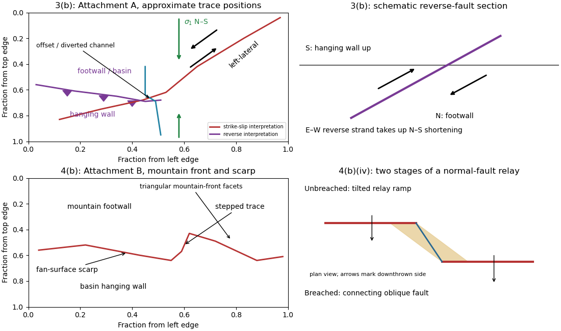
Original interpretive sketches for Attachments A and B, with normalized image positions and a normal-fault relay
. Details. 
A reverse fault can create a sharp mountain front by raising its hanging wall beside a lower footwall. Drainages entering the rising block may be deflected along the front or cut narrow gorges across it. In cross-section, draw a dipping fault with the hanging wall displaced up-dip and a surface-height contrast above the trace.
In Attachment A, mark the approximately east–west to west-northwest–east-southeast break between the southwestern mountain block and the central basin. Its approximate image coordinates run from through and to . The abrupt topographic change and diversion of drainage along this front support the reverse faulting interpretation. It is the southern margin of the central basin, not the much straighter oblique valley farther northeast. The original interpretive figure gives a schematic section.
Trace the strike-slip fault along the southwest–northeast valley, approximately through . The long oblique strand is interpreted as left-lateral strike-slip faulting: draw the southeastern side moving northeast and the northwestern side moving southwest, parallel to the trace.
This sense is consistent with horizontal north–south maximum compression: for an approximately northeast-striking fault, the resolved shear stress moves the southeastern side northeastward relative to the northwestern side. The deflected central drainage supports that interpretation. The regional stress direction supplies a consistency check rather than a uniquely precise trace location; follow the geomorphic break rather than drawing a single straight line through every coordinate.
Put the reverse fault along the mountain-front trace identified in part (ii), with the mountainous southern/southwestern block as hanging wall and the central basin to its north/northeast as footwall. Draw teeth on the southern hanging wall side of the line. In the simplest cross-section the fault dips south and the southern block moves northward and up over the basin edge. The image constrains the surface trace and relative uplift more securely than its subsurface fault dip; the precise dip cannot be measured from this map alone.
The network partitions deformation into oblique horizontal displacement on the strike-slip fault and more directly north–south crustal shortening on the approximately east–west reverse fault. On the oblique strand, northeastward motion of the southeastern side relative to the northwestern side has a northward component, reducing separation in the direction of . On the reverse fault, northward and upward motion of the southern hanging wall shortens and thickens the crust.
Sketch north–south opposing compression arrows around the plan view, left-lateral arrows along the oblique trace, and teeth on the southern side of the reverse fault trace. A section normal to the latter shows horizontal shortening converted into tectonic uplift. Where strands meet, folding, distributed strain or subsidiary faulting can maintain displacement compatibility; a strike-slip fault terminating abruptly in undeforming rock would not. This is an interpretation involving transpression, and the map does not by itself give a unique partition of slip rates between the strands.
Use repeat-pass interferometric synthetic-aperture radar. An orbiting radar transmits coherent microwave pulses and records the amplitude and phase of the returning field. Form an interferogram from registered complex images acquired before and after the earthquake, remove the orbital contribution and the topographic phase predicted by a digital elevation model, and correct atmospheric and other long-wavelength phase delays. Where interferometric coherence is adequate, unwrap the residual phase to estimate line-of-sight displacement:with sign set by the instrument's displacement convention. Each phase cycle represents of range change.
This maps a distributed earthquake displacement field day or night and through cloud, including areas inaccessible on foot. Roughly – ground sampling and a scene spanning many kilometres on both sides of the fault can resolve regional deformation; a narrow surface break benefits from finer pixels or complementary sub-metre optical surveys. Sensitivity to displacement can be millimetres to centimetres in coherent areas, but that does not equal spatial resolution. A single viewing direction measures one component; ascending and descending tracks and GNSS constrain more components. At the rupture itself, large gradients and changed ground cover can destroy interferometric coherence; radar pixel-offset tracking or before/after optical correlation can then recover metre-scale fault offsets.
Map the continuous break near the base of the rugged mountain front, following the low scarp across the smoother fan surfaces, rather than the ridgeline. With the same normalized image coordinates, an approximate trace follows , steps toward , and continues via . Some parts are much clearer than others and should be drawn as inferred or dashed where obscured.
The mountainous upper side of the image is the uplifted footwall; the smoother basin/fan side below is the downthrown hanging wall. A section perpendicular to the front has a normal fault dipping toward the basin. Attachment B has no printed north arrow, so these image-relative labels avoid assigning an unsupported compass direction. The original interpretive figure marks the trace and the central fault step-over.
Mark a fault scarp cutting an alluvial fan on the left-to-central smooth piedmont, approximately . Its narrow, aligned height break continues across surfaces that are smoother than the mountains; repeated downthrow on the basin side produces the scarp. Sketch a once-continuous gently sloping fan surface cut by a basin-facing step.
Mark triangular facets on the mountain front in the right-central part, near . These are roughly triangular planar mountain faces bounded laterally by incised valleys and below by the fault front. In a front view, draw repeated triangles separated by stream valleys. Triangular facets result from the interaction of normal faulting, uplift and erosion; neither they nor a sharp mountain front alone demonstrates a rupture in the particular historical event.
The rate of surface modification controls how quickly a fault scarp is erased. Strong rainfall, runoff, slope failure and easily eroded lithologies can round or dissect a scarp; dry conditions and resistant rock often preserve it longer. Alluvial fan deposition and aggradation can bury a scarp even if erosion is slow. A young marker surface can preserve an offset that an older, strongly modified surface no longer records.
The balance between fault slip rate, recurrence interval and marker age controls whether renewed displacement outruns this modification. Rapid or repeated normal faulting can maintain a clear front, whereas a long interval after a small displacement permits smoothing. A very young fan deposited after the event may have no offset, while an older surface may retain cumulative rather than single-event fault throw. These two controls explain why absence of an obvious scarp is not proof of an inactive fault.
An overlapping pair of basin-dipping normal fault segments can first accommodate displacement through an unbreached relay ramp. Fault throw tapers toward each tip and transfers between the strands; the intervening block tilts and bends while retaining a continuous ramp-like surface. Draw overlapping parallel traces in plan view and a tilted connecting surface between their different fault throws.
With continued extension, the ramp can be breached by a linking fault. An oblique connector joins the segment tips and takes up a combination of dip-slip and strike-slip displacement; the system becomes a more continuous, zigzag normal fault. Draw this connector diagonally through the overlap, with downthrown arrows on the basin side. Distributed small faults and folding can accompany either arrangement. The central bend around in Attachment B is the candidate transfer zone; the image alone does not uniquely establish the three-dimensional connection at depth.
Section C: Geophysical Methods.
A gravity anomaly is measured gravitational acceleration, reduced to a stated reference surface and compared with a reference gravity field. A local geological interpretation further removes or models the regional background. An absolute negative Bouguer gravity anomaly is therefore not itself a local negative geophysical density contrast.
Measure relative gravity with a calibrated gravimeter at stations across the profile, tie it to a base station, repeat base readings to estimate instrumental drift, and measure station coordinates and accurate elevations, for example by GNSS and levelling. Record observation times for tide corrections. Subtract the latitude-dependent reference gravity, correct instrument drift and Earth tides, add the free-air correction for station height, and subtract the attraction of the reference-density Bouguer slab. A terrain correction accounts for relief missing from or exceeding that slab. Use a consistent density such as for the topographic correction.[ref]
Geophysical Data Grids for the Conterminous United States by United States Geological Survey. Gravity anomaly reduction: free-air, simple-Bouguer and complete-Bouguer corrections
The question's reference to the anomaly in panel b is a panel-label slip: the upper plot contains gravity, while the lower plot supplies geometry and elevations. A geological slab thickness is the vertical thickness of the anomalous body, not simply its height above sea level.
For a laterally extensive Bouguer slab of thickness and geophysical density contrast ,The greenstone belt reaches from roughly to near its deepest central part, so use . The gravity maximum is approximately ; the exposed host-rock background in the south is approximately . Taking this as a constant regional reference gives a local excess . ThusThis is an approximate density under a constant-background, infinite-slab model. The finite width, variable thickness and neighboring pluton require a fuller gravity inversion for a precise value. In particular, the absolute value must not be inserted as the local excess.
Retain the same regional-background assumption as in part (b). The northern pluton is about thick beneath the station near the northern trough, while its gravity anomaly is about . Its anomaly relative to the greenstone maximum is approximately . Therefore the contrast equation isUsing the result of part (b), the second term contributes , leaving a net pluton anomaly of about . Hence , effectively close to the host-rock density at the precision of this diagram.
The apparent trough is strongly negative relative to the greenstone belt, but hardly negative relative to the southern host-rock background. If a northward regional trend is intended instead, it must be stated: in general,with both gravity values in milligals. For example, a northern background of would give , but the same reference would also change part (b). No regional curve is explicitly identified in the supplied figure, so the numerical result must retain its reference-field assumption. This is the geological nonuniqueness of geophysical inversion of potential-field interpretation, rather than a reason to force a presumed textbook granite density onto the plot.
Measure total magnetic field along the same south–north line with a calibrated magnetometer, recording position, time and sensor height. A simultaneous base-station magnetometer measures temporal variation so that diurnal changes can be removed from the moving survey. Avoid disturbed periods and magnetic contamination from vehicles, fences, power lines and equipment. Choose station spacing much smaller than the expected anomaly width, for example tens to hundreds of metres for a kilometre-scale target.
Subtract the epoch-appropriate International Geomagnetic Reference Field or another stated regional main-field model to obtain a total-field magnetic anomaly. Level overlapping traverses and remove offsets or drift where appropriate. Accurate terrain/sensor geometry is needed for comparison with a geological model, but there is no universal magnetic analogue of a constant-density Bouguer slab correction: the effect depends on the distribution and direction of magnetization. Measure magnetic susceptibility and remanent magnetization on representative greenstones, granite and host rock to test the assumed magnetic sources.
Assume the greenstone belt is more magnetically susceptible than the host rocks and granite, its magnetization is mainly induced magnetization, and the body is roughly east–west elongated so that the south–north line crosses it. At southern magnetic latitudes the main field has negative magnetic inclination in a north-and-down coordinate convention. The total-field magnetic anomaly is then generally asymmetric: the principal negative lobe is on the southern side and the positive lobe is displaced northward for the simple induced source illustrated here. The exact lobe sizes and peak positions depend on body geometry and the actual magnetic inclination.[ref]
Magnetic line profiles by UBC Geophysical Inversion Facility. Examples 1–2: the low lies north at northern inclination and south at southern inclination
An explicit sketching model is an induced magnetic dipole at depth . With northward coordinate , and unit field direction , its normalized total-field magnetic anomaly isThe plot uses only as an illustrative dipole-field inclination for a latitude near south, not a measured modern field at the site. A wide greenstone belt would broaden the response and can produce prominent edge anomalies. Remanent magnetization or a magnetic granite could change the sketch substantially; gravity alone cannot identify the magnetic source.
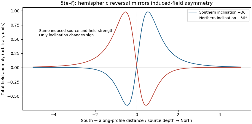
Induced-source magnetic anomalies for opposite inclinations on a south–north profile
. Details. 
For the same geometry, field strength and induced magnetization model at the opposite magnetic inclination, replacing by gives . Thus the north–south asymmetry reverses: the principal low moves to the northern side and the high to the southern side. It is a horizontal reflection of the simple profile, rather than a necessary reversal of every anomaly's sign. At a magnetic pole the induced anomaly is symmetric; at the magnetic equator the symmetry is different again. If remanent magnetization dominates, a hemisphere change alone does not determine the new profile because that remanence direction also has to be specified.
The sandstone records deposition of transported sand, followed by burial and cementation. For the Bunter setting, river channels, floodplains with channel sands and arid continental dune systems are plausible environments; a sandstone name alone does not uniquely distinguish them. Well-sorted or weakly cemented sand can retain the connected porosity and porous permeability needed for a saline aquifer.
The Zechstein evaporite suggests restricted marine basins or salinas in an arid climate, where evaporation concentrates seawater until dissolved salts precipitate. Repeated restriction and replenishment can build thick evaporite sequences, including rock salt. The Triassic limestone indicates carbonate accumulation, plausibly in warm, shallow marine settings with limited siliciclastic supply, followed by cementation. Some limestones can also form in lakes; the marine interpretation here uses the stated regional sequence.
Recommend a three-dimensional multichannel seismic reflection survey, with enough areal aperture, offsets and repeated coverage to image the reservoir top, base, structure and possible leakage faults. A two-dimensional reconnaissance line can be cheaper but cannot map a three-dimensional closure reliably and is vulnerable to out-of-plane reflections. Use seismic migration to position dipping reflectors and faults; repeatable acquisition is desirable if later carbon capture and storage monitoring is intended.
A tuned marine marine air-gun array supplies broadband low-frequency seismic wave energy that can penetrate to . Its trade-offs include bubble oscillations, seismic source ghosts, environmental constraints and limited high-frequency resolution. Sparker seismic source and boomer seismic source sources can provide higher-frequency, high-resolution shallow imaging, but commonly lack the energy and low frequencies needed to make them the first choice for this target. Source energy, bandwidth and repeatability must be balanced against penetration and vertical seismic resolution, approximately ; at and this is about . Required resolution ultimately depends on the unknown reservoir thickness.
A towed hydrophone streamer efficiently records pressure over many channels while a vessel moves. It primarily records P-wave pressure in the water, with flow noise, tow-depth ghosts, acquisition footprint and access restrictions as limitations. Seabed multicomponent nodes use hydrophones and geophones: pressure plus three-component ground motion can separate wavefields and recover converted S-wave information, and nodes permit wide azimuths and repeat surveys. Their costs include deployment, retrieval, coupling and positioning. Direct S waves do not propagate through the water column. The roughly water depth also creates a strong short-period water-layer seismic multiple that must be treated in processing.
Potential leakage paths are permeable or reactivated faults and connected fractures cutting the sealing sequence; lateral migration through connected reservoir layers into an unsealed outcrop or spill point; and natural or artificial penetrations such as poorly sealed abandoned wells or a compromised injection well. Injection raises pore pressure, potentially overcoming the capillary entry pressure of a seal, hydraulically opening fractures, or causing fault reactivation through reduced effective stress.
Seal continuity and porous permeability matter more than the rock name alone: a fractured or porous limestone need not be an effective caprock. Dissolution, chemical alteration or well-cement degradation can change leakage pathways over time. The underlying salt may be an effective barrier beneath the reservoir, but it does not seal the roof. Conversely, dissolved or residually trapped carbon dioxide is less mobile than a connected buoyant free-fluid phase, so connected porosity and fluid state also affect leakage.
For a horizontal interface, Snell law for elastic waves conserves horizontal seismic ray parameter . At the limestone–sandstone interface the incident P wave has . The reflected S wave remains in the limestone, sofrom vertical. All angles below use this normal-to-interface convention.
The transmitted P wave travels in the sandstone. Conservation of the seismic ray parameter givesIt bends toward the vertical because its seismic velocity is smaller.
For the transmitted S wave in sandstone, Snell law for elastic waves givesThe different transmitted P- and S-wave angles result from their different seismic velocities, despite their common horizontal seismic ray parameter.
Now reset the incident medium to sandstone; the new incident P wave has . Its reflected S wave hasThe equal result to part (d) follows from the equal ratio in the two incident layers.
For transmission into salt, , soThe transmitted P wave bends away from vertical because it enters a faster medium. The incident angle remains below the P-wave seismic critical angle at this interface.
Source notation assumption: the second printed is interpreted as . Otherwise the S-wave velocity in salt is not supplied, and this part and the salt S-wave calculations below would have no numerical answer. Retain the printed densities, including the unusually low salt value, rather than silently replacing them with typical rock properties.
With that interpretation, Snell law for elastic waves gives
A transmitted P-wave seismic head wave occurs when its refraction angle reaches , requiring . At the limestone–sandstone boundary the ratio is : there is no P-wave seismic critical angle for incidence from limestone. A slower lower layer cannot carry that transmitted head wave.
At the sandstone–salt boundary,The head wave travels along the faster salt boundary and radiates energy back into the slower overlying medium. Reversing the direction of incidence would change which interfaces admit such a head wave.
For a P-to-S converted seismic head wave, set the transmitted S-wave angle to , giving . At the limestone–sandstone boundary, , so no transmitted S-wave head wave is possible for incidence from limestone.
At the sandstone–salt boundary, using the stated interpretation ,The P-transmission seismic critical angle is lower, , but this does not forbid the converted S branch: at the transmitted P field is evanescent while the S field reaches grazing incidence.
P-wave seismic impedance is . In layer order limestone, sandstone, salt,The salt's larger P-wave seismic velocity is exactly offset by its smaller printed density, so the second interface has no P-wave seismic impedance contrast in this stipulated model.
S-wave seismic impedance is . With as documented in part (i),Unlike the P-wave case, the reservoir base has a nonzero S-wave seismic impedance contrast.
Specify the amplitude convention. For incident stress/pressure amplitude one, the normal-incidence seismic reflection coefficient and stress seismic transmission coefficient areAt limestone–sandstone, and . At sandstone–salt, and . The first return reverses the chosen stress-pulse polarity; the second interface produces no normal-incidence P return.
For a particle-velocity amplitude convention, and , giving and respectively. These are amplitude coefficients, not fractions of energy. The lossless reflected and transmitted energy fractions are and , which sum to one.
Apply the same stress-amplitude convention to S-wave seismic impedance. At limestone–sandstone,At sandstone–salt,A stress-amplitude transmission greater than one does not violate conservation of energy: the transmitted energy fraction includes the seismic impedance ratio. For particle velocity, the corresponding pairs are and . At normal incidence in isotropic layers, pure P and pure S waves do not undergo seismic mode conversion.
Let a positive incident stress wavelet be and measure return times relative to a receiver just above the reservoir. The top interface gives a negative P return of amplitude and no basal P return. For a separately generated and measured S wave, the top return is also negative, , while the basal return is positive, at the lower interface.
If is reservoir thickness, the basal return arrives or after the top return; no numerical is supplied. Including downward and upward transmission through the top boundary, but ignoring seismic attenuation, spreading and seismic multiples, its observed S-wave amplitude isThus the synthetic S trace has an earlier negative wavelet and a later, smaller positive wavelet; the synthetic P trace has only the earlier negative wavelet. The figure chooses solely to separate the pulses visually. Receiver electronics or a displacement convention can reverse the displayed trace polarity, so the convention must accompany the sketch.
A marine hydrophone streamer with a purely normal-incidence P source does not directly record the hypothetical S trace. A seabed multicomponent receiver and suitable S excitation or oblique-incidence seismic mode conversion are required. This distinguishes the calculated solid-layer response from what a particular acquisition system can measure.
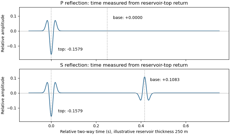
Idealized normal-incidence P and S reflection wavelets, including transmission through the reservoir top
. Details. 
Quality is degraded by vessel and flow noise, poor receiver coupling or position uncertainty, insufficient acquisition aperture and fold, coarse sampling and aliasing, and inaccurate source timing. Finite source bandwidth limits vertical seismic resolution; shallow-water reverberations, bubble pulses, source/receiver ghosts and seismic multiples overlap primary reflections. In of water with sound speed about , the water-layer round-trip time is only about .
Seismic attenuation removes high-frequency energy, geometric spreading weakens distant returns, and heterogeneous lithology, scattering and seismic anisotropy complicate travel paths and amplitudes. Incorrect seismic velocity models misplace reflectors during seismic migration; dipping structure and out-of-plane arrivals particularly challenge two-dimensional processing. Thin layers can cause wavelet interference and tuning. Finally, even noiseless data cannot recover a normal-incidence P reflection from the stipulated zero-contrast sandstone–salt boundary: that is absent signal rather than poor recording.
Section D: Thermodynamics.
For pure phases at the reference pressure , the Gibbs energy of reaction is . Chemical equilibrium requires , soThe reaction is muscovite dehydration to sanidine, corundum and water; its positive standard entropy of reaction makes the product assemblage favored at high temperature under this constant-property approximation.
Articles were limited to the first 100 out of 161 total.
Articles by others on the same topic
There are currently no matching articles.