Magnetization is magnetic dipole moment per unit volume, described by a vector field . Average the microscopic magnetic dipole moments in a small region of volume around the point :The averaging region should contain many microscopic constituents while being small compared with the distance over which the macroscopic magnetization varies. With number density of identical constituents, this becomes . Magnetic dipole moment has SI units , so magnetization has units : amperes per metre. The average is a vector sum, not a sum of magnitudes.[ref]
Magnetization. Classical Electromagnetism: An intermediate level course by Richard Fitzpatrick; Magnetization, equations (856)–(857) and the surrounding averaging definition
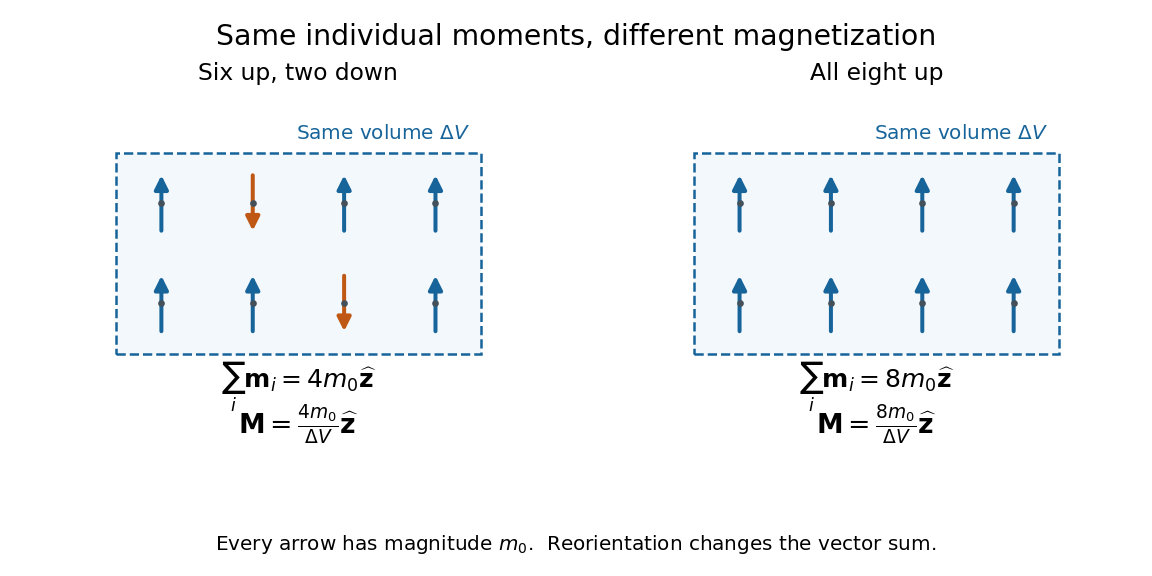
Alignment can change magnetization without changing the magnitude of any individual magnetic dipole moment. In a constructed counting example, eight equal magnetic dipole moments of magnitude occupy the same volume . Six along and two along give ; turning the two opposing magnetic dipole moments to doubles magnetization to . Both arrangements have the same sum of magnitudes, . Changing the individual magnetic dipole moments provides another possible response; their alignment and their magnitudes are distinct ingredients. Microscopic spin contributes magnetic dipole moment without being a literal rotating charged ball.
Distinguish magnetization , magnetic field , and magnetic field intensity . In SI,Here is the vacuum permeability, and denotes the tesla. Magnetization describes matter's magnetic dipole moment density; magnetic field enters the Lorentz force; magnetic field intensity separates the free electric current contribution in the macroscopic equations. In particular, zero applied magnetic field does not generally imply inside a finite magnet: its demagnetizing field depends on shape.[ref]
Magnetization. Classical Electromagnetism: An intermediate level course by Richard Fitzpatrick; Magnetization, equations (860)–(864): current decomposition and definition of H
For stationary electric polarization, magnetization produces bound current in the volume and on its bounding surface:The curl gives a current density in ; is a surface current density in . The unit normal points outward from the magnetized material into a region with zero magnetization. Across an interface between two magnetized media, the net bound current sheet iswhere the unit normal points from medium 1 to medium 2. Both faces contribute: medium 2 has the opposite outward normal vector. This fixes the cross product sign. If electric polarization changes with time, add its contribution to the bound current.[ref]
Permanent Ferromagnets. Classical Electromagnetism by Richard Fitzpatrick; Permanent Ferromagnets, equation (716): volume and outward-surface magnetization currents
A short proof outline explains why both contributions are needed. Write , where is the indicator function of the material's volume. In the sense of distributions, its gradient is , with the surface delta distribution. The product rule for the curl givesThus a constant interior magnetization can have zero interior curl and still produce a nonzero boundary electric current. Equivalently, neighboring ideal microscopic current loops cancel along shared edges while uncompensated edges remain on the outside. This bound current representation predicts the same macroscopic magnetic field as the magnetization distribution; it does not require a wire or free charge transport around the magnet. Its usefulness is that the familiar Biot-Savart law can now calculate the magnetic field from a specified magnetization.
A time-dependent average magnetization need not vary smoothly under a smooth drive. The Barkhausen effect resolves collective jumps through their induced electromotive force; Barkhausen pulse area explains how that derivative readout relates to the underlying change.
For a lattice spin system, magnetization density often means longitudinal spin per site, . A magnetic moment per physical volume instead includes the gyromagnetic conversion and lattice-site number density. The convention should be specified when comparing a spin-chain result with SI magnetization.
Magnetization measured after cooling without an applied field and then applying a measuring field. Comparison with field-cooled magnetization probes history dependence and slow relaxation.
Magnetization measured after cooling in an applied field, which can select magnetic domains or bias blocked moments.
Magnetic saturation is the regime in which increasing the applied magnetic field intensity produces little further increase in magnetization. The total magnetic flux density can still increase through its vacuum contribution, . Consequently a constant large magnetic permeability cannot describe a core throughout this regime; ideal magnetic circuit predictions based on that assumption overestimate field concentration.
Prescribe constant magnetization , with , inside a circular cylinder of radius and length , surrounded by zero magnetization. In cylindrical coordinates, the outward unit normal on the curved surface is , soThe endcaps have outward unit normals and . Their cross products with magnetization vanish, so on each endcap. The side bound current circulates counterclockwise when viewed from , by the right-hand rule. Zero endcap surface current density does not imply zero endcap magnetic field.
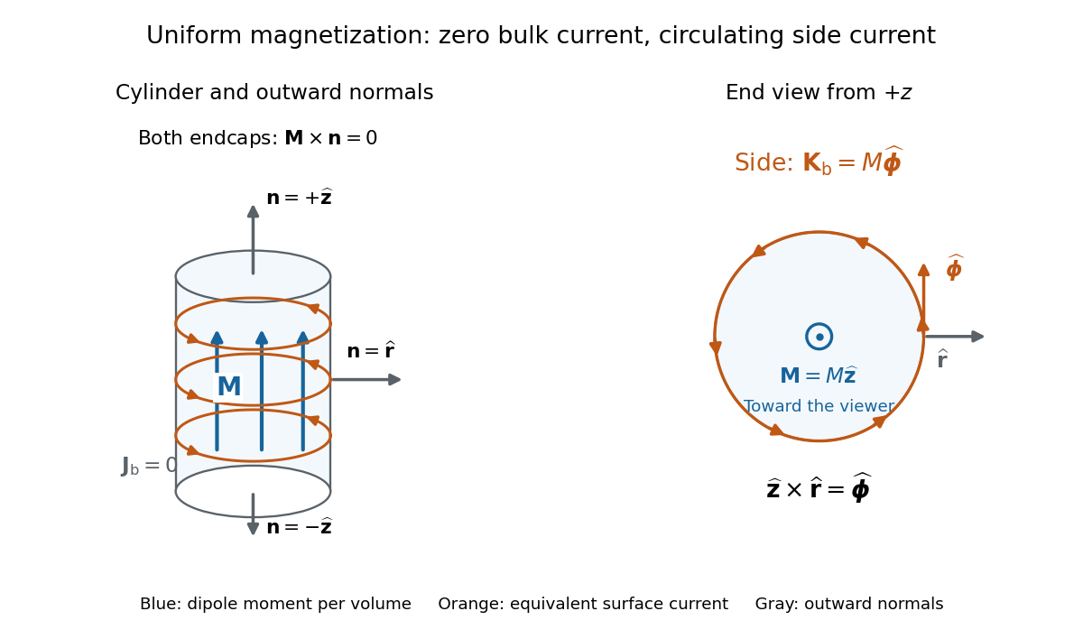
For an original example, let , , and . The volume and total magnetic dipole moment areCheck the result independently using the equivalent bound current: a side strip of axial length forms a current loop with and magnetic dipole moment . Its integral over gives the same . In particular, is the sum of the equivalent loop electric currents across a full axial cut; it is not a surface current density.
The side surface current density has exactly the geometry of a continuum solenoid with , where is solenoid turn density. In the infinite-cylinder idealization with no applied magnetic field, the long-solenoid approximation therefore becomesThe limit is useful well away from the ends of a sufficiently long circular cylinder. A finite circular cylinder instead has fringing magnetic field and a demagnetizing field. For this prescribed uniform magnetization, integrate the on-axis magnetic field of a circular current loop, or substitute in the on-axis magnetic field of a finite solenoid, to obtain the central magnetic field:Our example has and , rather than unity. With the rounded vacuum permeability , this is approximately , compared with the infinite-cylinder value . These are model calculations for a prescribed magnetization, not measured values or a solution for the self-consistent magnetization of an arbitrary material.
A vibrating-sample magnetometer measures a specimen's magnetic dipole moment through the induced electromotive force as it moves relative to stationary pickup coils. Dividing that magnetic dipole moment by the specimen's independently determined volume gives its average magnetization.
In Simon Foner's 1959 apparatus, the specimen was weighed and glued to a mount. A loudspeaker drive moved it perpendicular to an applied uniform magnetic field between magnet poles; stationary coils detected the induced electromotive force. A reference magnet on the same vibrating assembly generated a second coil electromotive force. Adjusting the reference voltage divider to an electrical null compared the specimen signal with this reference. The measurement calibration substituted a magnetically saturated pure nickel sphere of known magnetic dipole moment; a specimen-removed reading corrected the mount's contribution. The calibrated signal inferred the specimen's magnetic dipole moment, not its local magnetization map. Measurement uncertainty in the standard, positioning, finite specimen size, coil noise, and mechanical coupling limited the inference.[ref]
The readout follows Faraday's law of induction. In a small-displacement model with constant projected magnetic dipole moment , let the pickup-coil magnetic flux linkage be and the specimen motion be . Here incorporates coil geometry and turn count, is the displacement amplitude, and is angular frequency. To first order in displacement, with the derivative at the mean position,This is an original idealized readout relation: a larger induced electromotive force can mean larger magnetic dipole moment, greater motion, or a changed coil position. A synchronously moving reference allows common motion factors to cancel in the ratio of induced electromotive forces. The measurement calibration and specimen-removed control are therefore integral to the measurement. A single amplitude reading cannot by itself distinguish microscopic alignment from a change in individual magnetic dipole moments.
In a linear isotropic regime, a paramagnetic material has positive magnetic susceptibility: its induced magnetization is aligned with the applied magnetic field intensity. Molecular oxygen supplies an example discussed through molecular orbital theory in the covalent bond article.
A material exhibiting paramagnetism. Its induced magnetization points along the applied magnetic field in the linear-response regime, giving positive magnetic susceptibility. Unlike a ferromagnet, it has no spontaneous ordered moment in that phase. The inverse-temperature response of independent localized moments is one model, rather than a definition that includes all microscopic mechanisms of paramagnetism.
For independent magnetic moments constrained to , the one-site partition function is . The weak-field magnetization is , so the SI magnetic susceptibility obeys with . If , this involves , not the unrestricted-spin factor . The constraint on allowed moment orientations must be specified before using a Curie law coefficient.
At fixed positive temperature and weak field, independent spin- moments have total moment . This is the Curie law; the corresponding density divides by the sample volume.
For independent distinguishable moments with angular momentum , define . The one-site partition function is . Its logarithmic derivative gives . At this reduces to .
The Brillouin function gives the normalized magnetization of independent angular-momentum- moments. It is odd, increasing, has slope at zero and tends to at large positive or negative argument. Explicitly,It follows by differentiating the logarithm of , the one-ion partition function. Its limiting value gives magnetic saturation, and its initial slope gives the Curie law.
Paramagnetism arising when thermal excitation populates a magnetic manifold above a less magnetic or nonmagnetic ground manifold. Competing thermal population and orientational randomization can produce a maximum in susceptibility at an intermediate temperature.
The Curie–Weiss law approximates the magnetic susceptibility of interacting localized moments by in a suitable paramagnetic temperature range. A positive Weiss temperature often reflects predominantly ferromagnetic interactions, while a negative value often reflects antiferromagnetic interactions. It is not a universal exact law through an ordering transition, and crystal-field effects or itinerant carriers can require another description.
The fitted temperature in . It summarizes the leading high-temperature influence of interactions and need not equal the ordering temperature.
For independent localized two-state moments of projections along a field, the one-ion partition function is . Its thermal mean gives . A ion has , so the special value additionally assumes . At weak field the SI volume susceptibility is , neglecting demagnetizing corrections.
For moment projections , but , with . At zero field half the moments occupy each projection while the net magnetization is zero. An effective Curie moment is also distinct from the saturated projection used in this two-state model.
For independent moments with magnetic energies , and , where . This counts the magnetic orientations only, excluding translational and lattice entropy.
The Curie temperature is the transition temperature above which a ferromagnetic material loses spontaneous magnetization. A hot conducting planetary core can generate a magnetic field through dynamo action without behaving as a permanent magnet. The blocking temperature at which a mineral records crustal remanence also depends on its relaxation timescale and need not equal its Curie temperature.
Remanent magnetization is magnetization retained after the applied magnetic field has been removed. Magnetic minerals cooling in an ambient field can preserve information about that field in a planetary crust. Such a record may outlive the planetary dynamo which originally produced it. Crustal remanence therefore differs from a present field maintained by conducting-fluid motion.
A relativistic magnetization current has the form for an antisymmetric polarization-magnetization tensor. It is identically conserved because commuting derivatives contract an antisymmetric tensor.
Ferromagnetism is collective magnetic order with spontaneous magnetization below a Curie temperature. Interactions favor aligned magnetic moments; the Ising model represents a two-orientation version with positive coupling.
A magnetic domain can possess spontaneous magnetization even when other domains cancel its contribution to the whole specimen. Compare this spatial cancellation between domains with antiferromagnetism, where opposing magnetic sublattices compensate within the ordered structure, and ferrimagnetism, where their contributions are generally unequal. The magnetic sublattice diagram makes the three local patterns explicit.
Smoothly sweeping an applied magnetic field can reveal abrupt magnetization changes through the Barkhausen effect. A pickup coil detects the resulting changes of magnetic flux, making collective magnetic domain wall motion accessible as an electrical signal.
An itinerant mean-field model in which exchange splitting competes with the kinetic cost of unequal spin populations. Its instability condition is a suitably normalized interaction parameter times the Fermi-level density of states exceeding unity. It is distinct from a localized-spin exchange Hamiltonian for an insulator.
Formation of magnetic order with a spontaneous uniform magnetization. A large positive Pauli paramagnetism alone does not establish this: an instability caused by interactions is needed for spontaneous magnetization in zero applied magnetic field.
A hard magnetic material strongly resists reversal of its magnetization, giving high coercivity and useful remanence for permanent magnets. The relevant hardness is magnetic, not a mechanical strength rating.
A soft magnetic material changes its magnetization relatively easily and has a low coercive field. High useful permeability and small hysteresis losses favour such materials in electromagnets and alternating-field cores. “Soft” describes magnetic response rather than mechanical softness; electrically resistive ferrimagnets can also be magnetically soft.
A ferromagnet is a material that exhibits ferromagnetism. Its magnetic domains can cancel the net magnetization even while each domain remains ordered.
A magnetic domain is a region sharing an ordered magnetic orientation. Different magnetic domains can reduce the total magnetic moment without erasing the local magnetic order. A zero total magnetization therefore does not by itself establish antiferromagnetism.
A ferromagnetic particle with no internal domain wall. Magnetization reversal can proceed by rotation or nonuniform modes; thermal activation and anisotropy determine blocking and coercivity. Small size alone does not guarantee a permanent hard magnet.
A magnetic domain wall separates differently oriented magnetic domains. Its motion changes their volumes and average magnetization. It is a magnetic domain wall.
An original two-magnetic domain model makes the collective change explicit. Suppose opposite regions have magnetizations and along the measuring axis, where is the local saturation magnetization. If a magnetic domain wall sweeps volume from the negative region into the positive one, in a specimen of fixed volume , thenThe factor two comes from replacing by . The local magnitude stays fixed while the average magnetization changes; the event size depends on the swept volume, rather than a universal single-spin increment.
A trial domain pattern costs wall energy and can release stray energy . For a stable uniform ground state, within that trial model. Substituting the entire initial stray energy assumes that it is nearly all removed; a numerical lower bound independent of the domain geometry does not follow from single-domain observation alone.
Spatial variations in energy, including crystal defects, can trap a magnetic domain wall. This is magnetic domain-wall pinning. Increasing the applied magnetic field can release the wall into a collective jump.
The Barkhausen effect consists of abrupt magnetization changes during a smooth applied magnetic field sweep. Its inductive signal is Barkhausen noise, often arising from collective magnetic domain wall motion.[ref]
The distinction is between a smooth drive and an intermittent material response. A smooth macroscopic hysteresis curve can hide smaller jumps. By Faraday's law of induction, a pickup coil responds to the rate of change of linked magnetic flux, so a rapid jump can be conspicuous even when the total change is small. A pulse is not one chemical atom flipping: neither its height nor the number of audible clicks counts individual electron spins. Qualitative crackling alone does not establish quantum spin; collective switching also admits a classical model with trapped interfaces. Compare the distinct mechanical readout of angular momentum transfer in the Einstein-de Haas effect.
Heinrich Barkhausen's 1919 report used iron, a 300-turn pickup coil, moving magnet, amplified telephone readout and galvanometer. Removing iron corrected drive pickup. [ref]
The Barkhausen effect by Gianfranco Durin and Stefano Zapperi. Appendix A, p. 46: later translation of the 1919 apparatus and blank control
A modern primary experiment by Gianfranco Durin and Stefano Zapperi used annealed iron–silicon strips and amorphous alloys. A 60 cm solenoid swept a triangular magnetic field intensity; a 50-turn pickup coil, wound within 1 mm, sensed the specimen. A preamplifier with a 3–20 kHz low-pass filter preceded sampling. Measurements selected the central hysteresis region dominated by magnetic domain wall motion. Above-background threshold crossings defined event durations; integrating between crossings defined event sizes. These are reported procedures, rather than data generated for the diagrams.[ref]
Scaling exponents for Barkhausen avalanches in polycrystals and amorphous ferromagnets by Gianfranco Durin and Stefano Zapperi. pp. 1–2: apparatus, specimens and threshold integration
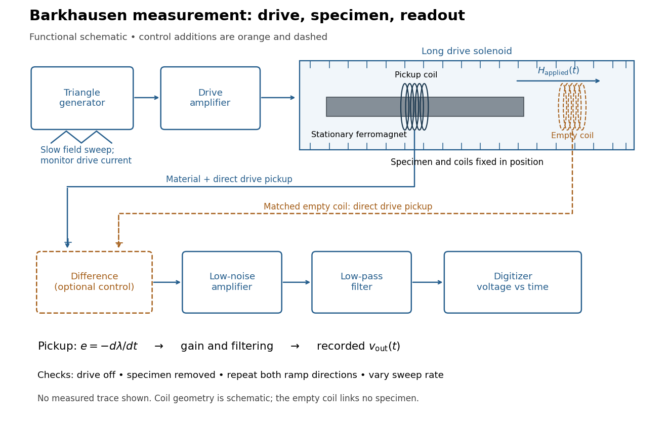
Barkhausen effect: swept magnetic field, stationary specimen and inductive readout
. Original functional schematic of the modern measurement principle. The specimen and pickup coil remain stationary; no torsional suspension or mechanical rotation is needed. The empty matching coil, difference stage and drive monitor show proposed controls, not an assertion that every component was present in the cited 2000 apparatus. The triangle indicates a drive waveform, not measured Barkhausen noise. Details.For this stationary implementation, secure a thin ferromagnet and its pickup coil inside a longer drive solenoid, keeping their relative positions fixed. Drive the solenoid with a slow triangular electric current, monitor that electric current, and record the amplified, filtered induced electromotive force with a digitizer. A speaker may make suitable frequencies audible, but the voltage record is needed for quantitative analysis. Slow variation of the drive does not require smooth magnetization. A triangular drive supplies an approximately constant applied-field sweep rate along each ramp; it does not guarantee constant instantaneous .
A proposed control sequence makes the inference testable. First record the electronics background with no drive. Repeat the same sweep with the specimen removed, retaining coil geometry: mutual induction from the drive can itself induce a voltage. A matching empty pickup coil wired in opposition can suppress common drive pickup, after checking its matching. Compensation of air flux by an opposed coil is an established method.[ref]
The Barkhausen effect by Gianfranco Durin and Stefano Zapperi. §II.A.1, p. 4: opposed-coil compensation
Then restore the specimen, repeat both sweep directions, reduce sweep rate, and compare the same hysteresis region with fixed amplifier gain, filter and threshold. Monitor drive irregularities and mechanical vibration; either can generate spurious pulses. These controls are recommendations for the schematic, rather than undocumented controls attributed to the modern paper.A genuine material contribution should differ from the blank-coil record and change reproducibly with the magnetic preparation and sweep region. Quieting the drive tests drive-correlated pickup, but a held field need not eliminate all delayed material motion. Reversing the sweep is a consistency check on signed changes, not a demand that individual events retrace. A changing pulse count under a different filter or threshold cannot by itself establish changed microscopic dynamics. The useful inference is intermittent collective magnetization change within the instrument's signal bandwidth, with spatial detail left unresolved.
Write the magnetic flux linkage of the stationary pickup coil as , in SI units of weber. If every turn links the same magnetic flux , then ; the turn count is dimensionless. With a fixed winding and terminal convention, Faraday's law of induction gives the induced electromotive forceThis is the fundamental theorem of calculus applied to magnetic flux linkage. Its units are , not volts alone. Reversing the leads reverses the sign. In a high-input-electrical resistance voltage measurement the input approximately follows this electromotive force; coil loading and the frequency response of the electronics require separate calibration.
Separate direct drive linkage from material linkage: . Even an empty pickup coil has . In an ideal long, uniformly coupled specimen with negligible demagnetizing field correction and eddy current shielding, a useful material approximation isHere is specimen cross-sectional area, not the larger coil aperture; is vacuum permeability and the axial magnetization sampled by the coil. The units check directly: . Finite geometry and nonuniform magnetization generally require a calibrated coupling in place of . The exact linkage identity survives that failure of the uniform approximation.
As an original illustrative calculation, stipulate , , and rounded . ThenA uniform change over would give a rectangular pulse of ; over it gives with the same area. Thus pulse height mixes change size with change speed. These numbers describe an ideal model, not observed pulses or material constants.
An explicit constructed model separates slow magnetization drift from discrete collective jumps:Here is the Heaviside step function, the Dirac delta function, a smooth drift rate, and the jump times. The ideal discontinuities stand for events shorter than the resolved timescale; actual magnetic domain walls move over finite times. This equation stipulates jump sizes rather than deriving them from atomic spin. With in the preceding geometry, subtracting the smooth background leaves .
Let a stable linear filter have causal impulse response , normalized by , and let be a constant dimensionless voltage gain. The output is a convolution:A simple low-pass filter has , with time constant . Its output pulse has peak proportional to and signed area . Integrating the convolution proves area preservation because ; a wider filter response lowers peaks and lengthens tails. This ideal filter models resolution, rather than claiming the cited instrument had exactly this response.

The nearby positive jumps in the figure have additive negative pulse areas even when their tails overlap. For the first of the pair still has of its initial height when the second arrives. Thresholding can merge those responses into one detected event; limited signal bandwidth also obscures their separation. The total signed area still records the sum if the complete response is integrated, but cannot identify how that sum was partitioned into events. Equal simultaneous jumps are exactly indistinguishable from a single jump of their summed size in this linear measurement. Oppositely signed simultaneous changes can cancel.
Area preservation requires the stated electronics. A zero-DC stage after the low-pass filter has responseConsequently over the complete response: a main pulse is followed by a compensating tail. Integrating only a threshold-selected lobe, clipping the record, or saturating the amplifier breaks the simple pulse-area inference. Recovering a magnetization change from such a readout needs the calibrated frequency response and an appropriate reconstruction. Neither the audible crackle nor the displayed voltage is a direct staircase of magnetization.
Articles by others on the same topic



Magnetization refers to the vector field that expresses the magnetic moment per unit volume of a material. It is a measure of how much a material responds to an applied magnetic field and is used to understand its magnetic properties.