Past exam of the year 2 of the earth sciences (geology) course of the University of Oxford / 2024 / Paper 3 / 2

A gravity anomaly is the difference between observed gravitational acceleration and a specified reference prediction after defined reductions. A free-air gravity anomaly, a Bouguer gravity anomaly, and a residual local gravity anomaly differ because they remove different reference contributions. State the reference ellipsoid, datum, reference density, and regional trend before interpreting an anomaly as a subsurface geophysical density contrast.

On land, tie gravimeter observations to a gravity base, calibrate them, correct instrumental drift and Earth tides, and determine station latitude and elevation accurately. Subtract latitude-dependent normal gravity $\gamma (\phi )$. Reduce to the reference elevation using a positive free-air correction for a station above that datum: about $+0.3086h\mathrm{mGal}$ for $h$ in metres. A simple Bouguer gravity anomaly then subtracts attraction of the intervening rock slab and adds the conventional terrain correction:with all acceleration terms expressed consistently. In SI units $1\mathrm{mGal}=10^{-5}\mathrm{m}{\mathrm{s}}^{-2}$.

At sea, also correct vessel-motion effects, especially the Eötvös correction from east–west vessel motion and Earth rotation, and vertical ship acceleration; average or filter the moving-platform data appropriately. GPS navigation and tide information specify position and measurement height. Sea-surface measurements give a marine free-air gravity anomaly after motion, latitude, tide and height reductions. A marine Bouguer gravity anomaly additionally allows for measured bathymetry and the replacement of low-density water by reference rock; the simple water-column replacement correction is positive, $2\pi G({\rho }_{\mathrm{ref}}-{\rho }_w)H$, relative to the sea-surface free-air value. A consistent three-dimensional bathymetric correction is preferable near irregular coasts. Remove a justified broad regional field if the intended quantity is a residual anomaly of the local body.

For a wide horizontal Bouguer slab replacing surrounding basement, use the density contrast $\Delta \rho ={\rho }_{\mathrm{sed}}-{\rho }_{\mathrm{base}}$, not the absolute sediment density:Take downward attraction as positive. The negative anomaly therefore requires $\Delta \rho <0$. With $\Delta g=-40\mathrm{mGal}=-4.0\times 10^{-4}\mathrm{m}{\mathrm{s}}^{-2}$, $h=3000\mathrm{m}$, and $G=6.67430\times 10^{-11}{\mathrm{m}}^3\mathrm{k}{\mathrm{g}}^{-1}{\mathrm{s}}^{-2}$,soThis is the requested Bouguer slab approximation: a flat observation surface, laterally infinite constant-thickness material, uniform average geophysical density contrast, and a regional anomaly already removed. The actual basin in Figure 1 narrows downwards and is finite. For a fixed maximum thickness, finite width reduces the central anomaly magnitude, so this calculation can underestimate the true magnitude of the average geophysical density contrast. It does not establish a unique basement density without the geometrical assumption.

Use the same surrounding basement density inferred in solution, carrying its unrounded value through the arithmetic. The intrusion's geophysical density contrast isThe Bouguer slab thickness needed to produce the same negative peak is thereforeThe smaller absolute geophysical density contrast requires a thicker body. This is an approximate vertical thickness and, if the top is close to the surface as drawn in Figure 1, an approximate base depth below that top. It is not an independent estimate of the intrusion's burial depth. For an infinite slab the anomaly does not depend on top depth; a buried top would require additional geometry. Finite width and the downward-widening outline in Figure 1 make 8 km a slab-equivalent estimate rather than a uniquely determined geological depth.

For the two negative gravity anomalies in the actual Figure 1, examine where the steepest flanks occur within the total fall into the trough. The solid upper intrusion profile has maximum slope relatively low on its flanks, close to the flat trough; its body widens downwards. The lower basin profile has maximum slope relatively high on its flanks, near the shoulders; its body narrows downwards. The dashed gradient traces and arrows mark these transitions. The signed derivative changes sign on opposite sides of a symmetric trough; a plot of gradient magnitude instead gives two positive peaks.

A shallow edge controls a relatively abrupt local change, whereas deeper geophysical density contrast spreads its effect over greater horizontal distance. Downward-narrowing geometry leaves relatively more of the anomaly associated with the shallow broad part, placing the strong flank change nearer the outer shoulders. Downward-widening geometry adds a broader deep contribution beneath the narrow outcrop, shifting the inflection towards the lower part of the trough. Thus the location of a flank's maximum slope relative to its shoulder and minimum is more useful here than the shared $-40\mathrm{mGal}$ peak alone.

A symmetric constant-density body with vertical sides gives a symmetric negative trough with paired rounded flanks; for a broad shallow body the main slope changes occur approximately halfway down those flanks. It is intermediate between the two end members, rather than a triangular anomaly or a rectangular discontinuity. Exact fractional inflection heights depend on width, depth, burial and rounding. The following independently calculated infinite-strike models illustrate the distinction without copying Figure 1.

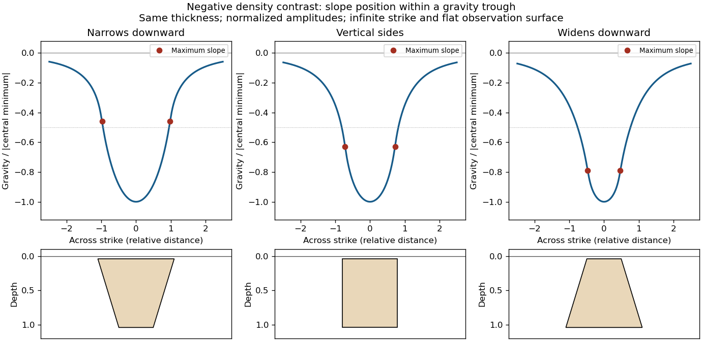
This qualitative inference assumes approximately comparable simple bodies, uniform geophysical density contrast, and a properly removed regional field. Gravity inversion is non-unique: lateral density changes, multiple bodies, and a buried top can imitate changes of wall slope. Use the seismic reflection constraints to test the interpretation.

Assume that the intrusion has a positive magnetic susceptibility contrast, that induced magnetization dominates its remanent magnetization, and that the local present-day geomagnetic field points roughly northward and downward, as in this northern mid-latitude setting. Writewhere $\mathbf{b}$ is the anomalous magnetic field and the last expression assumes $|\mathbf{b}|\ll |{\mathbf{B}}_0|$. A total-field magnetic anomaly measures a field projection, so it need not have the same sign everywhere above a high-susceptibility body.^[ref]

The 100 km east–west extent makes an approximately two-dimensional, east–west-striking body a useful model away from its ends. On a profile drawn north on the left, south on the right, the expected normally induced response has a subsidiary negative lobe on the northern side and a stronger positive lobe over the body, displaced towards the south. The northward horizontal field component makes the anomaly asymmetric; its downward component produces the dominant positive response. The field falls back towards the regional value away from the intrusion. Broad bodies can have edge shoulders or a broad central high, so the sketch represents a qualitative shape rather than one uniquely specified curve.

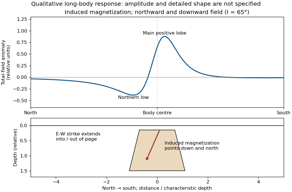
An exactly vertical inducing field would remove this north–south skew for a symmetric induced body. Real magnetic inclination and magnetic declination should be taken from a suitable geomagnetic field model for the survey date and location; no exact local value is supplied here. Strong oblique or reversed remanent magnetization can shift or reverse the lobes, and heterogeneous magnetic susceptibility, body dip and three-dimensional end effects can alter the profile. Higher magnetic susceptibility alone does not determine a unique amplitude or polarity pattern without these qualifications.